6
$\begingroup$

How does one plot the set S of parameter region of equations using r?. My problem is that I have one equation with 2 variables defined by $g(x,a,b) = 0$ and I want to plot the set of $(a,b)$ where the solution exists.

The specific example I am interested in is the following:

$$(F(x) - a)f^2(x) + \left(\frac{F^2(x)}{2} - a F(x) + \left(\frac{a^2}{2} + b\right)\right)f^\prime(x)=0.$$

where $F$ is the cumulative function of a normal distribution of mean=0 and sd=1, $f$ the density function of the normal, and $f^\prime$ is the first derivative of $f$.

My goal is to construct the region (surface) $S$ where

$$S = \{(a,b)\in [0,1]^2\ |\text{ a solution }x\text{ of the equation exists and belongs to }[0,1]\}. $$

E<-function(a,u) {  
((a-u)*(dnorm(q(u),m,s, log = FALSE))/(qnorm(u)))-((qnorm(u))^2)/2 +a*qnorm(u)-(a^2)/2 
}
a <- u <- seq(0,1,0.01)
z <- outer(a,u,E)
b<-seq(0,1,0.001)
contour( x=a, y=a, z=z,levels=b, las=1, drawlabels=FALSE, lwd=3,xlab="a", ylab="x")

Please help me here. I hope this can teach me more. Thanks in advance.


Thanks, this is exactly what I was looking for. But I have 2 remarks or comments : Remark 1 : I made a mistake $u=F(x)\in[0,1]$ but $x = N(0,1)$ so $x$ is not restricted in $[0,1]$. So is it possible for you to propose the code that you used in Mathematica such that I can try to adapt it.

Remark 2 : I did also a simulation using Mathematica and I get the 3D picture of my equation but it was not possible to get the projection to get S. This is the code I used :

f[u_] := Quantile[NormalDistribution[0, 1], u]
g[u_]:=PDF[NormalDistribution[0,1],f[u]]
h[u_, a_, e_] := (u - a)*((g[u])^2) + ((u^2)/2 - a*u + (a^2)/2 + e)*f[u]*g[u]
ContourPlot3D[h[u, a, e] == 0, {a, 0, 1}, {u, 0, 1}, {e, 0, 1}]

Then I get this picture :
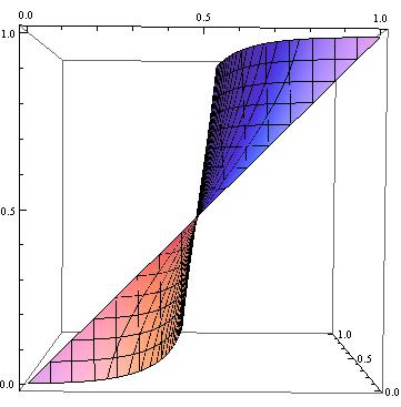
enter image description here

So is there way to get the projection from this picture.

$\endgroup$

1 Answer 1

5
$\begingroup$

To address the general question, consider using a tool that is well adapted to such calculations and visualizations, such as Mathematica. (This was used to plot the first two and last two figures below.)

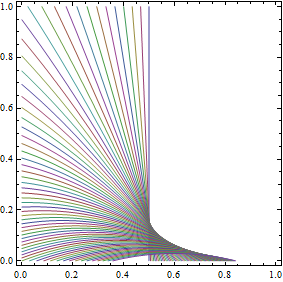
This particular question is amenable to further analysis which enables R to display $S$: for each $x\in [0,1]$, we can plot the subset of $S$ it determines (which is a curve). By choosing a visually dense collection of such $x$, the collection of these curves limns the entire region $S$.


Begin the analysis by rewriting the defining equation in the form

$$b = -\frac{1}{2} a^2 + u(x) a + v(x)$$

where (assuming $x\ne 0$)

$$u(x) = f(x)^2/f^\prime(x) + F(x)$$ and $$v(x) = -\left(F(x) f(x)^2/f^\prime(x) + \frac{1}{2}F(x)^2\right).$$

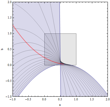
In the $(a,b)$ plane these equations describe similar parabolae having their vertexes at $(u(x), v(x) + u(x)^2/2).$

Figure 1

In this figure some of the parabolae are drawn in gray. The locus of their vertexes is traced by the thick red curve. The region $[0,1]\times [0,1]$ is shown as a gray square. $S$ is the portion of the gray square overlapped by the shaded blue region.

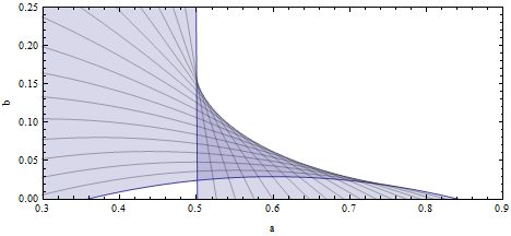
The region $S$ comprises most of the left half of the unit square ($a\le 1/2$), less a small region at the bottom, together with pieces of some parabolae at the bottom. The next figure examines that lower region in more detail.

Figure 2

The piece missing from $S$ in the left half of the unit square lies below the parabola $b = -\frac{1}{2}a^2 + u(1)a + v(1)\approx -\frac{1}{2}a^2 + 0.599374 a - 0.15035.$ The part of $S$ in the right half of the unit square (where the curves seem to overlap) is bounded by the envelope of these parabolae; it is difficult to derive any simple formula for its boundary.


R code

Begin with a function f to compute values along a parabola given by $x \ne 0$:

f <- function(a, x) {
  F <- pnorm(x)
  f0 <- dnorm(x)
  f1 <- -x * exp(-x^2 / 2) / sqrt(2 * pi)
  return(-1/2 * a^2 + (f0^2/f1 + F)*a - (F*f0^2/f1 + F^2/2))
}

Because interest lies in $0\le a\le 1$, a typically will be a sequence of numbers in this range; f returns the ordinates of the parabola lying above this sequence.

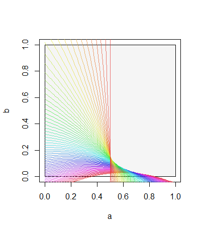
Use this iteratively to draw the parabolae. The vertical line $a=\frac{1}{2}$ (corresponding to $x=0$) needs to be drawn separately because it is not the graph of a function of $a$.

n.mesh <- 64
mesh <- seq(0, 1, length.out=n.mesh)
colors <- hsv(mesh, .8, .9, 2/3)
plot(c(0,1), c(0,1), type="n", xlab="a", ylab="b")
rect(0,0,1,1, col=gray(0.96))

for(i in n.mesh:2) {
  x0 <- mesh[i]
  curve(f(x, x0), add=TRUE, col=colors[i])
}
abline(v=1/2, xlim=c(0,1), ylim=c(0,1), col=colors[1])

Figure 3


Appendix: Brute Force Code

In Mathematica a brute-force (but somewhat efficient) way to find a subset of $S$, when the function $x\to g(x,a,b)$ is continuous for all $(a,b)\in[0,1]^2$, checks whether this function changes sign between $x=0$ and $x=1$. Begin by defining $g$:

fF[x_] := CDF[NormalDistribution[], x];
f[x_] := PDF[NormalDistribution[]][x];
f1[x_] := Evaluate[D[f[y], y] /. y -> x];
g[x_, a_, b_] := (fF[x] - a) f[x]^2 + (fF[x]^2/2 - a fF[x] + (a^2/2 + b)) f1[x];

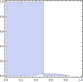
Here is the solution (which plots quickly):

RegionPlot[g[0, a, b] g[1, a, b] < 0 , {a, 0, 1}, {b, 0, 1}]

Figure 3

In general some analysis is required to assure that this covers all of $S$. That analysis can be assisted by plotting contours of $(a,b)\to g(x,a,b)$ for various values of $x$ of interest:

ContourPlot[Evaluate@Table[g[x, a, b] == 0, {x, Range[0, 1, 1/64]}], {a, 0, 1}, {b, 0, 1}]

Figure 4

To the extent you can trust R to produce accurate contour plots, a similar solution is available for it.

$\endgroup$
0

Your Answer

By clicking “Post Your Answer”, you agree to our terms of service and acknowledge you have read our privacy policy.

Not the answer you're looking for? Browse other questions tagged or ask your own question.