Is there an elegant/insightful way to understand this linear regression identity for multiple $R^2$?

Question

In linear regression I have come across a delightful result that if we fit the model

$$E[Y] = \beta_1 X_1 + \beta_2 X_2 + c,$$

then, if we standardize and centre the $Y$, $X_1$ and $X_2$ data,

$$R^2 = \mathrm{Cor}(Y,X_1) \beta_1 + \mathrm{Cor}(Y, X_2) \beta_2.$$

This feels to me like a 2 variable version of $R^2 = \mathrm{Cor}(Y,X)^2$ for $y=mx+c$ regression, which is pleasing.

But the only proof I know is not in anyway constructive or insightful (see below), and yet to look at it it feels like it should be readily understandable.

Example thoughts:

• The $\beta_1$ and $\beta_2$ parameters give us the 'proportion' of $X_1$ and $X_2$ in $Y$, and so we are taking respective proportions of their correlations...
• The $\beta$s are partial correlations, $R^2$ is the squared multiple correlation... correlations multiplied by partial correlations...
• If we orthogonalize first then the $\beta$s will be $\mathrm{Cov}/\mathrm{Var}$... does this result make some geometric sense?

None of these threads seem to lead anywhere for me. Can anyone provide a clear explanation of how to understand this result.

---

Unsatisfying Proof

\begin{equation} R^2 = \frac{SS_{reg}}{SS_{Tot}} = \frac{SS_{reg}}{N} = \langle(\beta_1 X_1 + \beta_2 X_2)^2\rangle \\= \langle\beta_1^2 X_1^2\rangle + \langle\beta_2^2 X_2^2\rangle + 2\langle\beta_1\beta_2X_1X_2\rangle \end{equation}

and

\begin{equation} \mathrm{Cor}(Y,X_1) \beta_1 + \mathrm{Cor}(Y, X_2) \beta_2 = \langle YX_1\rangle\beta_1 + \langle Y X_2\rangle \beta_2\\ =\langle \beta_1 X_1^2 + \beta_2 X_1 X_2\rangle \beta_1 + \langle \beta_1 X_1 X_2 + \beta_2 X_2^2\rangle \beta_2\\ =\langle \beta_1^2 X_1^2\rangle + \langle \beta_2^2 X_2^2 \rangle + 2\langle \beta_1 \beta_2 X_1 X_2\rangle \end{equation}

QED.

Answer 1

The following three formulas are well known, they are found in many books on linear regression. It is not difficult to derive them.

$\beta_1= \frac {r_{YX_1}-r_{YX_2}r_{X_1X_2}} {\sqrt{1-r_{X_1X_2}^2}}$

$\beta_2= \frac {r_{YX_2}-r_{YX_1}r_{X_1X_2}} {\sqrt{1-r_{X_1X_2}^2}}$

$R^2= \frac {r_{YX_1}^2+r_{YX_2}^2-2 r_{YX_1}r_{YX_2}r_{X_1X_2}} {\sqrt{1-r_{X_1X_2}^2}}$

If you substitute the two betas into your equation $R^2 = r_{YX_1} \beta_1 + r_{YX_2} \beta_2$, you will get the above formula for R-square.

---

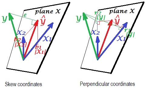
Here is a geometric "insight". Below are two pictures showing regression of $Y$ by $X_1$ and $X_2$. This kind of representation is known as variables-as-vectors in subject space (please read what it is about). The pictures are drawn after all the three variables were centered, and so (1) every vector's length = st. deviation of the respective variable, and (2) angle (its cosine) between every two vectors = correlation between the respective variables.

$\hat{Y}$ is the regression prediction (orthogonal projection of $Y$ onto "plane X"); $e$ is the error term; $cos \angle{Y \hat{Y}}={|\hat Y|}/|Y|$, multiple correlation coefficient.

The left picture depicts skew coordinates of $\hat{Y}$ on variables $X_1$ and $X_2$. We know that such coordinates relate the regression coefficients. Namely, the coordinates are: $b_1|X_1|=b_1\sigma_{X_1}$ and $b_2|X_2|=b_2\sigma_{X_2}$.

And the right picture shows corresponding perpendicular coordinates. We know that such coordinates relate the zero order correlation coefficients (these are cosines of orthogonal projections). If $r_1$ is the correlation between $Y$ and $X_1$ and $r_1^*$ is the correlation between $\hat Y$ and $X_1$ then the coordinate is $r_1|Y|=r_1\sigma_{Y} = r_1^*|\hat{Y}|=r_1^*\sigma_{\hat{Y}}$. Likewise for the other coordinate, $r_2|Y|=r_2\sigma_{Y} = r_2^*|\hat{Y}|=r_2^*\sigma_{\hat{Y}}$.

So far it were general explanations of linear regression vector representation. Now we turn for the task to show how it may lead to $R^2 = r_1 \beta_1 + r_2 \beta_2$.

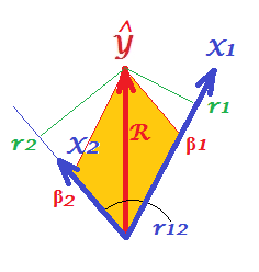
First of all, recall that in their question @Corone put forward the condition that the expression is true when all the three variables are standardized, that is, not just centered but also scaled to variance 1. Then (i.e. implying $|X_1|=|X_2|=|Y|=1$ to be the "working parts" of the vectors) we have coordinates equal to: $b_1|X_1|=\beta_1$; $b_2|X_2|=\beta_2$; $r_1|Y|=r_1$; $r_2|Y|=r_2$; as well as $R=|\hat Y|/|Y|=|\hat Y|$. Redraw, under these conditions, just the "plane X" of the pictures above:

On the picture, we have a pair of perpendicular coordinates and a pair of skew coordinates, of the same vector $\hat Y$ of length $R$. There exist a general rule to obtain perpendicular coordinates from skew ones (or back): $\bf P = S C$, where $\bf P$ is points X axes matrix of perpendicular ones; $\bf S$ is the same sized matrix of skew ones; and $\bf C$ are the axes X axes symmetric matrix of angles (cosines) between the nonorthogonal axes.

$X_1$ and $X_2$ are the axes in our case, with $r_{12}$ being the cosine between them. So, $r_1 = \beta_1 + \beta_2 r_{12}$ and $r_2 = \beta_1 r_{12} + \beta_2$.

Substitute these $r$s expressed via $\beta$s in the @Corone's statement $R^2 = r_1 \beta_1 + r_2 \beta_2$, and you'll get that $R^2 = \beta_1^2 + \beta_2^2 + 2\beta_1\beta_2r_{12}$, - which is true, because it is exactly how a diagonal of a parallelogram (tinted on the picture) is expressed via its adjacent sides (quantity $\beta_1\beta_2r_{12}$ being the scalar product).

This same thing is true for any number of predictors X. Unfortunately, it is impossible to draw the alike pictures with many predictors.

Please see similar pictures in this great answer.

Answer 2

The hat matrix is idempotent.

(This is a linear-algebraic way of stating that OLS is an orthogonal projection of the response vector onto the space spanned by the variables.)

---

Recall that by definition

$$R^2 = \frac{ESS}{TSS}$$

where

$$ESS = (\hat Y)^\prime \hat Y$$

is the sum of squares of the (centered) predicted values and

$$TSS = Y^\prime Y$$

is the sum of squares of the (centered) response values. Standardizing $Y$ beforehand to unit variance also implies

$$TSS = Y^\prime Y = n.$$

Recall, too, that the estimated coefficients are given by

$$\hat\beta = (X^\prime X)^{-} X^\prime Y,$$

whence

$$\hat Y = X \hat \beta = X (X^\prime X)^{-} X^\prime Y = H Y$$

where $H$ is the "hat matrix" effecting the projection of $Y$ onto its least squares fit $\hat Y$. It is symmetric (which is obvious from its very form) and idempotent. Here is a proof of the latter for those unfamiliar with this result. It's just shuffling parentheses around:

$$\eqalign{H^\prime H = H H &=\left( X (X^\prime X)^{-} X^\prime\right)\left(X (X^\prime X)^{-} X^\prime \right) \\ &= X (X^\prime X)^{-} \left(X^\prime X \right) (X^\prime X)^{-} X^\prime \\ &= X (X^\prime X)^{-} X^\prime = H. }$$

Therefore

$$R^2 = \frac{ESS}{TSS} = \frac{1}{n} (\hat Y)^\prime \hat Y = \frac{1}{n}Y^\prime H^\prime H Y = \frac{1}{n}Y^\prime H Y = \left(\frac{1}{n}Y^\prime X\right) \hat \beta.$$

The crucial move in the middle used the idempotence of the hat matrix. The right hand side is your magical formula because $\frac{1}{n}Y^\prime X$ is the (row) vector of correlation coefficients between $Y$ and the columns of $X$.