Simulate from a dynamic mixture of distributions

Question

I need to sample from the following mixture of two distributions:

$h_{\vec{\beta}}(r)=c(\vec{\beta})[(1-w_{m,\tau}(r))f_{\vec{\beta_{0}}}(r)+w_{m,\tau}(r)g_{\epsilon,\sigma}(r)]$

where $c(\vec{\beta})$ is a normalizing constant, $f_{\vec{\beta_{0}}}$ is the Gamma distribution, $g_{\epsilon,\sigma}$ is the Generalized Pareto distribution, and $w_{m,\tau}$ is the CDF of the Cauchy distribution: $1/2 +(1/\pi)*arctan[(r-m)/\tau]$, acting here as a weight/mixing function providing a smooth transition between the Gamma and Pareto (hence the adjective "dynamic" to qualify the mixture).

The weights allow having one unified mixture where the Gamma captures the bulk of the data, and as we get closer to the extremes, the Pareto takes over control. The approach originated in Figressi et al. (2002), and I have adopted the implementation presented in Vrac and Naveau (2007).

I have estimated the parameters $\vec{\beta}=(m,\tau,\gamma,\lambda,\epsilon,\xi)$, respectively the location and scale of the Cauchy CDF, shape and rate of the Gamma, and shape and scale of the GPD, following the procedure based on MLE described in the second paper referenced (R code can be found here), and now I want to sample from $h_{\vec{\beta}}$. Since the proportions of each component of the mixture are not fixed, I cannot just randomly sample from one distribution or the other (e.g., using using the rgamma() or rgpd() R functions) like is done here or here. So, how should I proceed?

If I could determine the CDF of the mixture, I could use inversion sampling ($U(0,1)$). EDIT: as noted by Xi'an in the second thread listed right below there is no closed form solution for the CDF.

EDIT: implementation of one of the two strategies in Xi'an's answer (rejection sampling) for my data here and Monte Carlo approach to estimating the quantile function of the mixture here.

Answer 1

As pointed out by Dougal, the shape of your target density$$h_\beta(r)\propto (1-w_{m,\tau}(r))f_{\beta_0}(r)+w_{m,\tau}(r) g_{\epsilon,\sigma}(r) $$is open to accept-reject simulation since $$(1-w_{m,\tau}(r))f_{\beta_0}(r)+w_{m,\tau}(r) g_{\epsilon,\sigma}(r) \le f_{\beta_0}(r)+g_{\epsilon,\sigma}(r)=2\left\{\frac{1}{2}f_{\beta_0}(r)+\frac{1}{2}g_{\epsilon,\sigma}(r)\right\} $$ Therefore simulating from the even mixture of Pareto $f_{\beta_0}$ and Gamma $g_{\epsilon,\sigma}$ and accepting with probability $$\dfrac{(1-w_{m,\tau}(r))f_{\beta_0}(r)+w_{m,\tau}(r) g_{\epsilon,\sigma}(r)}{f_{\beta_0}(r)+g_{\epsilon,\sigma}(r)}$$ would return you an exact output from your target density.

Note that the original paper by Frigessi et al. does include a way to simulate from the dynamic mixture on page 6: with probability $1/2$ simulate from $f_{\beta_0}$ and with probability $1/2$ from $g_{\epsilon,\sigma}$ [which is equivalent to simulating from the even mixture] and accept the outcome with probability $1-w_{m,\tau}(r)$ in the first case and $w_{m,\tau}(r)$ in the second case. It is unclear which one of those approaches has the highest average acceptance rate.

Here is a small experiment that shows the acceptance rates are comparable:

#Frigessi et al example
beta=2
lambda=gamma(1.5)
mu=tau=1
xi=.5
sigma=1
#the target is 
target=function(x) 
(1-pcauchy((x-mu)/tau))*dweibull(x,shape=beta,scale=1/lambda)+pcauchy((x-mu)/tau)*dgpd(x,xi=xi,beta=sigma)[1]

T=1e4
u=sample(c(0,1),T,rep=TRUE)
x=u*rweibull(T,shape=beta,scale=1/lambda)+(1-u)*rgpd(T,xi=xi,beta=sigma)
#AR 1
ace1=mean(runif(T)<(u*(1-pcauchy((x-mu)/tau))+(1-u)*pcauchy((x-mu)/tau)))
#AR 2
ace2=mean(runif(T)<target(x)/(dweibull(x,shape=beta,scale=1/lambda)+dgpd(x,xi=xi,beta=sigma)[1]))

with

> ace1
[1] 0.5173
> ace2
[1] 0.5473

An alternative is to use a Metropolis-Hastings algorithm. For instance, at each iteration of the Markov chain,

1. pick the Pareto against the Gamma components with probabilities $1-w_{m,\tau}(x^{t-1})$ and $w_{m,\tau}(x^{t-1})$;
2. Generate a value $y$ from the chosen component;
3. Accept the value $y$ as $x^t=y$ with probability $$\dfrac{(1-w_{m,\tau}(y))f_{\beta_0}(y)+w_{m,\tau}(y) g_{\epsilon,\sigma}(y)}{(1-w_{m,\tau}(x^{t-1}))f_{\beta_0}(x^{t-1})+w_{m,\tau}(x^{t-1}) g_{\epsilon,\sigma}(x^{t-1})}$$ $$\times\dfrac{(1-w_{m,\tau}(y))f_{\beta_0}(x^{t-1})+w_{m,\tau}(y) g_{\epsilon,\sigma}(x^{t-1})}{(1-w_{m,\tau}(x^{t-1}))f_{\beta_0}(y)+w_{m,\tau}(x^{t-1}) g_{\epsilon,\sigma}(y)}$$ otherwise take $x^t=x^{t-1}$

The corresponding R code is straightforward

#MCMC style
propose=function(x,y){
#moving from x to y
target(y)*(pcauchy((y-mu)/tau,lowe=FALSE)*dweibull(x,shape=beta,scale=1/lambda)+pcauchy((y-mu)/tau)*dgpd(x,xi=xi,beta=sigma)[1:length(x)])/
(target(x)*(pcauchy((x-mu)/tau,lowe=FALSE)*dweibull(y,shape=beta,scale=1/lambda)+pcauchy((x-mu)/tau)*dgpd(y,xi=xi,beta=sigma)[1:length(x)]))}

x=seq(rgpd(1,xi=xi,beta=sigma),T)
for (t in 2:T){
  #proposal
  x[t]=rweibull(1,shape=beta,scale=1/lambda)
  if (runif(1)<pcauchy((x[t-1]-mu)/tau)) x[t]=rgpd(1,xi=xi,beta=sigma)
  #acceptance
  if (runif(1)>propose(x[t-1],x[t])) x[t]=x[t-1]}
ace3=length(unique(x))/T

and gives a higher acceptance rate

> ace3
[1] 0.877

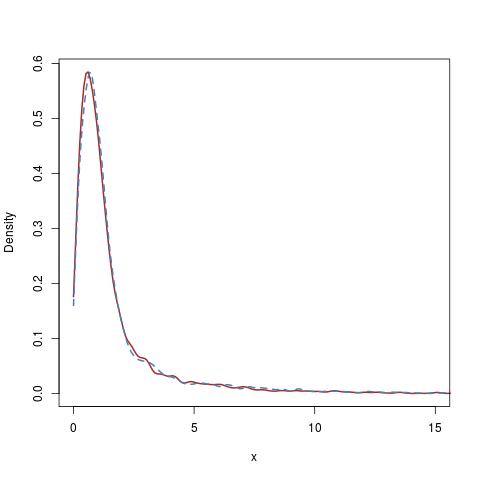
While the fit is identical to the density estimate obtained by accept-reject:

[Red curve for the accept-reject sample and blue curve for the MCMC sample, both based on 10⁴ original simulations]

Answer 2

I suggest that you investigate Probabilistic Programming. Basically, you write programs that operate on probability distributions rather than (random) variables. This makes it easy to define functions that are dynamic mixtures of distributions. While full-featured Probabilistic Programming systems support Bayesian statistical inference, your application doesn't really need it. Primarily you just need the programming language and the Markov Chain Monte Carlo (MCMC) solvers to generate samples from the distribution defined by your program.

Good introductions and list of resources can be found in the following:

• http://radar.oreilly.com/2013/04/probabilistic-programming.html
• http://probabilistic-programming.org/wiki/Home

Good tutorials on Probabilistic Programming can be found at the Church web site, especially the second, "Simple Generative Models":

• http://projects.csail.mit.edu/church/wiki/Cornell_tutorial
• http://projects.csail.mit.edu/church/wiki/Simple_Generative_Models

Finally, investigate STAN as an implementation platform. There are versions for R and Python. Again, you just need the generative model capabilities.