replaced http://stats.stackexchange.com/ with https://stats.stackexchange.com/
Source Link

I don’t really get what you mean with AGWN, is this simply that $n(t_i)$ are independent with $n(t_i) \sim N(0,\sigma^2)$?

The least squares estimator (which, as usual with a normal model, coincide with maximum likelihood estimator, see eg this answerthis answer) is easy to find with numerical methods, here is a piece of R code:

a <- 2; b <- 0.2; c <- -1
t <- seq(-5,10, length=100)
y <- a*exp(-b*t)+c+rnorm(length(t), sd=2)
f <- function(par, t, y) { 
  a <- par[1]; b <- par[2]; c <- par[3]; 
  return(sum((a*exp(-b*t)+c-y)**2 ) ); }
nlm( function(par) f(par, t, y), c(0,0,0))

The result of the last call is

$minimum
[1] 430.8242

$estimate
[1]  2.0875336  0.1961210 -0.8672079

$gradient
[1]  1.301591e-05 -2.745537e-05  2.603429e-05

$code
[1] 1

$iterations
[1] 19

Our initial values (2, 0.2, -1) are estimated by (2.088, 0.196, -0.867). You can get a plot of the data points, the "true model" (red line) and the estimated model (dotted red line) as follows:

plot(t,y)
lines( t, a*exp(-b*t)+c, col="red")
nlm( function(par) f(par, t, y), c(0,0,0))$estimate -> r
lines( t, r[1]*exp(-r[2]*t)+r[3], col="red", lty=2)
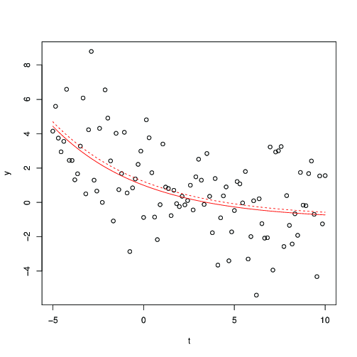
Data points, with in red line the true model, in dotted red line the fitted model

Also, be sure not to miss this related questionthis related question already quoted by whuber in the comments.

A few hints for numerical optimization

In the above code the numerical optimization is done using nlm, a function of R. Here are a few hints for a more elementary solution.

If $b\ne 0$ is fixed, it is easy to find $a$ and $c$ minimizing $f(a,b,c) = \sum_{i=1}^n (a \exp(-b\cdot t_i) +c -y_i)^2$: this a the classical least squares for the linear model. Namely, letting $x_i = \exp(-b\cdot t_i)$, we find $$ \begin{array}{rcccl} a &=& a(b) &=& { n \sum_i y_i x_i - \left( \sum_i y_i \right)\left(\sum_i x_i \right)\over n \sum x_i^2 - \left(\sum_i x_i \right)^2 }, \\ c &=& c(b) &=& { \sum_i y_i \sum_i x_i^2 - \left( \sum_i y_i x_i \right)\left(\sum_i x_i \right)\over n \sum x_i^2 - \left(\sum_i x_i \right)^2 }. \\ \end{array}$$

Then set $$ g(b) = f(a(b), b, c(b)).$$ The optimization problem is now reduced to find the minimum of $g(b)$. This can be done either using Newton method or a ternary search.

I don’t really get what you mean with AGWN, is this simply that $n(t_i)$ are independent with $n(t_i) \sim N(0,\sigma^2)$?

The least squares estimator (which, as usual with a normal model, coincide with maximum likelihood estimator, see eg this answer) is easy to find with numerical methods, here is a piece of R code:

a <- 2; b <- 0.2; c <- -1
t <- seq(-5,10, length=100)
y <- a*exp(-b*t)+c+rnorm(length(t), sd=2)
f <- function(par, t, y) { 
  a <- par[1]; b <- par[2]; c <- par[3]; 
  return(sum((a*exp(-b*t)+c-y)**2 ) ); }
nlm( function(par) f(par, t, y), c(0,0,0))

The result of the last call is

$minimum
[1] 430.8242

$estimate
[1]  2.0875336  0.1961210 -0.8672079

$gradient
[1]  1.301591e-05 -2.745537e-05  2.603429e-05

$code
[1] 1

$iterations
[1] 19

Our initial values (2, 0.2, -1) are estimated by (2.088, 0.196, -0.867). You can get a plot of the data points, the "true model" (red line) and the estimated model (dotted red line) as follows:

plot(t,y)
lines( t, a*exp(-b*t)+c, col="red")
nlm( function(par) f(par, t, y), c(0,0,0))$estimate -> r
lines( t, r[1]*exp(-r[2]*t)+r[3], col="red", lty=2)

Data points, with in red line the true model, in dotted red line the fitted model

Also, be sure not to miss this related question already quoted by whuber in the comments.

A few hints for numerical optimization

In the above code the numerical optimization is done using nlm, a function of R. Here are a few hints for a more elementary solution.

If $b\ne 0$ is fixed, it is easy to find $a$ and $c$ minimizing $f(a,b,c) = \sum_{i=1}^n (a \exp(-b\cdot t_i) +c -y_i)^2$: this a the classical least squares for the linear model. Namely, letting $x_i = \exp(-b\cdot t_i)$, we find $$ \begin{array}{rcccl} a &=& a(b) &=& { n \sum_i y_i x_i - \left( \sum_i y_i \right)\left(\sum_i x_i \right)\over n \sum x_i^2 - \left(\sum_i x_i \right)^2 }, \\ c &=& c(b) &=& { \sum_i y_i \sum_i x_i^2 - \left( \sum_i y_i x_i \right)\left(\sum_i x_i \right)\over n \sum x_i^2 - \left(\sum_i x_i \right)^2 }. \\ \end{array}$$

Then set $$ g(b) = f(a(b), b, c(b)).$$ The optimization problem is now reduced to find the minimum of $g(b)$. This can be done either using Newton method or a ternary search.

that's it... (hints for optimization)
Source Link
Elvis
  • 12.9k
  • 43
  • 59

I don’t really get what you mean with AGWN, is this simply that $n(t_i)$ are independent with $n(t_i) \sim N(0,\sigma^2)$?

The least squares estimator (which, as usual with a normal model, coincide with maximum likelihood estimator, see eg this answer) is easy to find with numerical methods, here is a piece of R code:

a <- 2; b <- 0.2; c <- -1
t <- seq(-5,10, length=100)
y <- a*exp(-b*t)+c+rnorm(length(t), sd=2)
f <- function(par, t, y) { 
  a <- par[1]; b <- par[2]; c <- par[3]; 
  return(sum((a*exp(-b*t)+c-y)**2 ) ); }
nlm( function(par) f(par, t, y), c(0,0,0))

The result of the last call is

$minimum
[1] 430.8242

$estimate
[1]  2.0875336  0.1961210 -0.8672079

$gradient
[1]  1.301591e-05 -2.745537e-05  2.603429e-05

$code
[1] 1

$iterations
[1] 19

Our initial values (2, 0.2, -1) are estimated by (2.088, 0.196, -0.867). You can get a plot of the data points, the "true model" (red line) and the estimated model (dotted red line) as follows:

plot(t,y)
lines( t, a*exp(-b*t)+c, col="red")
nlm( function(par) f(par, t, y), c(0,0,0))$estimate -> r
lines( t, r[1]*exp(-r[2]*t)+r[3], col="red", lty=2)

Data points, with in red line the true model, in dotted red line the fitted model

Also, be sure not to miss this related question already quoted by whuber in the comments.

A few hints for numerical optimization

In the above code the numerical optimization is done using nlm, a function of R. Here are a few hints for a more elementary solution.

If $b\ne 0$ is fixed, it is easy to find $a$ and $c$ minimizing $f(a,b,c) = \sum_{i=1}^n (a \exp(-b\cdot t_i) +c -y_i)^2$: this a the classical least squares for the linear model. Namely, letting $x_i = \exp(-b\cdot t_i)$, we find $$ \begin{array}{rcccl} a &=& a(b) &=& { n \sum_i y_i x_i - \left( \sum_i y_i \right)\left(\sum_i x_i \right)\over n \sum x_i^2 - \left(\sum_i x_i \right)^2 }, \\ c &=& c(b) &=& { \sum_i y_i \sum_i x_i^2 - \left( \sum_i y_i x_i \right)\left(\sum_i x_i \right)\over n \sum x_i^2 - \left(\sum_i x_i \right)^2 }. \\ \end{array}$$

Then set $$ g(b) = f(a(b), b, c(b)).$$ The optimization problem is now reduced to find the minimum of $g(b)$. This can be done either using Newton method or a ternary search.

I don’t really get what you mean with AGWN, is this simply that $n(t_i)$ are independent with $n(t_i) \sim N(0,\sigma^2)$?

The least squares estimator (which, as usual with a normal model, coincide with maximum likelihood estimator, see eg this answer) is easy to find with numerical methods, here is a piece of R code:

a <- 2; b <- 0.2; c <- -1
t <- seq(-5,10, length=100)
y <- a*exp(-b*t)+c+rnorm(length(t), sd=2)
f <- function(par, t, y) { 
  a <- par[1]; b <- par[2]; c <- par[3]; 
  return(sum((a*exp(-b*t)+c-y)**2 ) ); }
nlm( function(par) f(par, t, y), c(0,0,0))

The result of the last call is

$minimum
[1] 430.8242

$estimate
[1]  2.0875336  0.1961210 -0.8672079

$gradient
[1]  1.301591e-05 -2.745537e-05  2.603429e-05

$code
[1] 1

$iterations
[1] 19

Our initial values (2, 0.2, -1) are estimated by (2.088, 0.196, -0.867). You can get a plot of the data points, the "true model" (red line) and the estimated model (dotted red line) as follows:

plot(t,y)
lines( t, a*exp(-b*t)+c, col="red")
nlm( function(par) f(par, t, y), c(0,0,0))$estimate -> r
lines( t, r[1]*exp(-r[2]*t)+r[3], col="red", lty=2)

Data points, with in red line the true model, in dotted red line the fitted model

Also, be sure not to miss this related question already quoted by whuber in the comments.

A few hints for numerical optimization

In the above code the numerical optimization is done using nlm, a function of R. Here are a few hints for a more elementary solution.

If $b\ne 0$ is fixed, it is easy to find $a$ and $c$ minimizing $f(a,b,c) = \sum_{i=1}^n (a \exp(-b\cdot t_i) +c -y_i)^2$: this a the classical least squares for the linear model. Namely, letting $x_i = \exp(-b\cdot t_i)$, we find $$ \begin{array}{rcccl} a &=& a(b) &=& { n \sum_i y_i x_i - \left( \sum_i y_i \right)\left(\sum_i x_i \right)\over n \sum x_i^2 - \left(\sum_i x_i \right)^2 }, \\ c &=& c(b) &=& { \sum_i y_i \sum_i x_i^2 - \left( \sum_i y_i x_i \right)\left(\sum_i x_i \right)\over n \sum x_i^2 - \left(\sum_i x_i \right)^2 }. \\ \end{array}$$

Then set $$ g(b) = f(a(b), b, c(b)).$$ The optimization problem is now reduced to find the minimum of $g(b)$. This can be done either using Newton method or a ternary search.

+ref to question/answer about MLE / LSE
Source Link
Elvis
  • 12.9k
  • 43
  • 59

I don’t really get what you mean with AGWN, is this simply that $n(t_i)$ are independent with $n(t_i) \sim N(0,\sigma^2)$?

Least square areThe least squares estimator (which, as usual with a normal model, coincide with maximum likelihood estimator, see eg this answer) is easy to find with numerical methods, here is a piece of R code:

a <- 2; b <- 0.2; c <- -1
t <- seq(-5,10, length=100)
y <- a*exp(-b*t)+c+rnorm(length(t), sd=2)
f <- function(par, t, y) { 
  a <- par[1]; b <- par[2]; c <- par[3]; 
  return(sum((a*exp(-b*t)+c-y)**2 ) ); }
nlm( function(par) f(par, t, y), c(0,0,0))

The result of the last call is

$minimum
[1] 430.8242

$estimate
[1]  2.0875336  0.1961210 -0.8672079

$gradient
[1]  1.301591e-05 -2.745537e-05  2.603429e-05

$code
[1] 1

$iterations
[1] 19

Our initial values (2, 0.2, -1) are estimated by (2.088, 0.196, -0.867). You can get a plot of the data points, the "true model" (red line) and the estimated model (dotted red line) as follows:

plot(t,y)
lines( t, a*exp(-b*t)+c, col="red")
nlm( function(par) f(par, t, y), c(0,0,0))$estimate -> r
lines( t, r[1]*exp(-r[2]*t)+r[3], col="red", lty=2)

Data points, with in red line the true model, in dotted red line the fitted model

Also, be sure not to miss this related question already quoted by whuber in the comments.

I don’t really get what you mean with AGWN, is this simply that $n(t_i)$ are independent with $n(t_i) \sim N(0,\sigma^2)$?

Least square are easy with numerical methods, here is piece of R code:

a <- 2; b <- 0.2; c <- -1
t <- seq(-5,10, length=100)
y <- a*exp(-b*t)+c+rnorm(length(t), sd=2)
f <- function(par, t, y) { 
  a <- par[1]; b <- par[2]; c <- par[3]; 
  return(sum((a*exp(-b*t)+c-y)**2 ) ); }
nlm( function(par) f(par, t, y), c(0,0,0))

The result of the last call is

$minimum
[1] 430.8242

$estimate
[1]  2.0875336  0.1961210 -0.8672079

$gradient
[1]  1.301591e-05 -2.745537e-05  2.603429e-05

$code
[1] 1

$iterations
[1] 19

Our initial values (2, 0.2, -1) are estimated by (2.088, 0.196, -0.867). You can get a plot of the data points, the "true model" (red line) and the estimated model (dotted red line) as follows:

plot(t,y)
lines( t, a*exp(-b*t)+c, col="red")
nlm( function(par) f(par, t, y), c(0,0,0))$estimate -> r
lines( t, r[1]*exp(-r[2]*t)+r[3], col="red", lty=2)

Data points, with in red line the true model, in dotted red line the fitted model

I don’t really get what you mean with AGWN, is this simply that $n(t_i)$ are independent with $n(t_i) \sim N(0,\sigma^2)$?

The least squares estimator (which, as usual with a normal model, coincide with maximum likelihood estimator, see eg this answer) is easy to find with numerical methods, here is a piece of R code:

a <- 2; b <- 0.2; c <- -1
t <- seq(-5,10, length=100)
y <- a*exp(-b*t)+c+rnorm(length(t), sd=2)
f <- function(par, t, y) { 
  a <- par[1]; b <- par[2]; c <- par[3]; 
  return(sum((a*exp(-b*t)+c-y)**2 ) ); }
nlm( function(par) f(par, t, y), c(0,0,0))

The result of the last call is

$minimum
[1] 430.8242

$estimate
[1]  2.0875336  0.1961210 -0.8672079

$gradient
[1]  1.301591e-05 -2.745537e-05  2.603429e-05

$code
[1] 1

$iterations
[1] 19

Our initial values (2, 0.2, -1) are estimated by (2.088, 0.196, -0.867). You can get a plot of the data points, the "true model" (red line) and the estimated model (dotted red line) as follows:

plot(t,y)
lines( t, a*exp(-b*t)+c, col="red")
nlm( function(par) f(par, t, y), c(0,0,0))$estimate -> r
lines( t, r[1]*exp(-r[2]*t)+r[3], col="red", lty=2)

Data points, with in red line the true model, in dotted red line the fitted model

Also, be sure not to miss this related question already quoted by whuber in the comments.

added 28 characters in body
Source Link
Elvis
  • 12.9k
  • 43
  • 59
Loading
Source Link
Elvis
  • 12.9k
  • 43
  • 59
Loading