deleted 1832 characters in body
Source Link
Antoni Parellada
  • 26.9k
  • 18
  • 122
  • 230

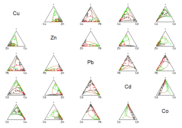
I've been trying to reproduce this matrix scatter plots, and understand them. For instance, I had trouble calling the multiple plots with the curves around points of the grouping categorical variable:

> levels(sa.groups.area)
[1] "Lower"  "Middle" "Upper" 

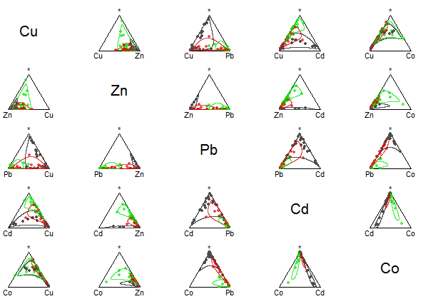
Finally, though, I got a practically identical plot with this code:

library(compositions)
data(SimulatedAmounts)
colors = c(rgb(red=0.3, green=0.3,  blue=.3, alpha=1),
           rgb(red=0.9, green=0,    blue=0, alpha=0.7),
           rgb(red=0,   green=.9,   blue=0, alpha=0.7))

tt = acomp(sa.groups5)
plot(tt, col = rgb(0,0,0,0), bg = colors[as.numeric(sa.groups.area)], pch = 21, cex = .9)

strata = sa.groups5.area
temp = cbind(sa.groups5,strata)

a = acomp(temp[temp[ , 6] == 1, ][,1:5])
ellipses(mean(a), var(a), r = 2, col = colors[1])

b = acomp(temp[temp[ , 6] == 2, ][,1:5])
ellipses(mean(b), var(b), r = 2, col = colors[2])

c = acomp(temp[temp[ , 6] == 3, ][,1:5])
ellipses(mean(c), var(c), r = 2, col = colors[3])

enter image description here


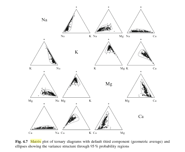
In Analyzing Compositional Data with R By K. Gerald van den Boogaart, Raimon Tolosana-Delgado the following plot can be found with a telling caption:

enter image description here

and (minimally) paraphrasing:

in which the radius of the lines contain 95% of the probability assuming a normal model for the composition and a known variance.

The code of this latter plot likely includes the lines:

r = sqrt(qchisq(p = .095, df = 2))
mm = mean(tt)
vr = var(tt)
ellipses(mean = mm, var = vr, r = r)

... and ?ellipses describes the r parameter in the function ellipses as:

r      a scaling of the half-diameters

The remaining question is:

What are the meaning and mathematics behind these deformed circles (lines or curves) generated by the function ellipses, and how to generate them?

I've been trying to reproduce this matrix scatter plots, and understand them. For instance, I had trouble calling the multiple plots with the curves around points of the grouping categorical variable:

> levels(sa.groups.area)
[1] "Lower"  "Middle" "Upper" 

Finally, though, I got a practically identical plot with this code:

library(compositions)
data(SimulatedAmounts)
colors = c(rgb(red=0.3, green=0.3,  blue=.3, alpha=1),
           rgb(red=0.9, green=0,    blue=0, alpha=0.7),
           rgb(red=0,   green=.9,   blue=0, alpha=0.7))

tt = acomp(sa.groups5)
plot(tt, col = rgb(0,0,0,0), bg = colors[as.numeric(sa.groups.area)], pch = 21, cex = .9)

strata = sa.groups5.area
temp = cbind(sa.groups5,strata)

a = acomp(temp[temp[ , 6] == 1, ][,1:5])
ellipses(mean(a), var(a), r = 2, col = colors[1])

b = acomp(temp[temp[ , 6] == 2, ][,1:5])
ellipses(mean(b), var(b), r = 2, col = colors[2])

c = acomp(temp[temp[ , 6] == 3, ][,1:5])
ellipses(mean(c), var(c), r = 2, col = colors[3])

enter image description here


In Analyzing Compositional Data with R By K. Gerald van den Boogaart, Raimon Tolosana-Delgado the following plot can be found with a telling caption:

enter image description here

and (minimally) paraphrasing:

in which the radius of the lines contain 95% of the probability assuming a normal model for the composition and a known variance.

The code of this latter plot likely includes the lines:

r = sqrt(qchisq(p = .095, df = 2))
mm = mean(tt)
vr = var(tt)
ellipses(mean = mm, var = vr, r = r)

... and ?ellipses describes the r parameter in the function ellipses as:

r      a scaling of the half-diameters

The remaining question is:

What are the meaning and mathematics behind these deformed circles (lines or curves) generated by the function ellipses?

The question is:

What are the meaning and mathematics behind these deformed circles (lines or curves) generated by the function ellipses, and how to generate them?
deleted 65 characters in body
Source Link
Antoni Parellada
  • 26.9k
  • 18
  • 122
  • 230
library(compositions)
data(SimulatedAmounts)
colors = c(rgb(red=0.3, green=0.3,  blue=.3, alpha=1),
           rgb(red=0.9, green=0,    blue=0, alpha=0.7),
           rgb(red=0,   green=.9,   blue=0, alpha=0.7))
           
tt = acomp(sa.groups5)
plot(tt, col = rgb(0,0,0,0), bg = colors[as.numeric(sa.groups.area)], pch = 21, cex = .9)
ellipses(mean(tt), var(tt), r = 2, col = "peru")

strata = sa.groups5.area
temp = cbind(sa.groups5,strata)

a = acomp(temp[temp[ , 6] == 1, ][,1:5])
ellipses(mean(a), var(a), r = 2, col = colors[1])

b = acomp(temp[temp[ , 6] == 2, ][,1:5])
ellipses(mean(b), var(b), r = 2, col = colors[2])

c = acomp(temp[temp[ , 6] == 3, ][,1:5])
ellipses(mean(c), var(c), r = 2, col = colors[3])

enter image description hereenter image description here

library(compositions)
data(SimulatedAmounts)
colors = c(rgb(red=0.3, green=0.3,  blue=.3, alpha=1),
           rgb(red=0.9, green=0,    blue=0, alpha=0.7),
           rgb(red=0,   green=.9,   blue=0, alpha=0.7))
           
tt = acomp(sa.groups5)
plot(tt, col = rgb(0,0,0,0), bg = colors[as.numeric(sa.groups.area)], pch = 21, cex = .9)
ellipses(mean(tt), var(tt), r = 2, col = "peru")

strata = sa.groups5.area
temp = cbind(sa.groups5,strata)

a = acomp(temp[temp[ , 6] == 1, ][,1:5])
ellipses(mean(a), var(a), r = 2, col = colors[1])

b = acomp(temp[temp[ , 6] == 2, ][,1:5])
ellipses(mean(b), var(b), r = 2, col = colors[2])

c = acomp(temp[temp[ , 6] == 3, ][,1:5])
ellipses(mean(c), var(c), r = 2, col = colors[3])

enter image description here

library(compositions)
data(SimulatedAmounts)
colors = c(rgb(red=0.3, green=0.3,  blue=.3, alpha=1),
           rgb(red=0.9, green=0,    blue=0, alpha=0.7),
           rgb(red=0,   green=.9,   blue=0, alpha=0.7))

tt = acomp(sa.groups5)
plot(tt, col = rgb(0,0,0,0), bg = colors[as.numeric(sa.groups.area)], pch = 21, cex = .9)

strata = sa.groups5.area
temp = cbind(sa.groups5,strata)

a = acomp(temp[temp[ , 6] == 1, ][,1:5])
ellipses(mean(a), var(a), r = 2, col = colors[1])

b = acomp(temp[temp[ , 6] == 2, ][,1:5])
ellipses(mean(b), var(b), r = 2, col = colors[2])

c = acomp(temp[temp[ , 6] == 3, ][,1:5])
ellipses(mean(c), var(c), r = 2, col = colors[3])

enter image description here

added 592 characters in body
Source Link
Antoni Parellada
  • 26.9k
  • 18
  • 122
  • 230

SoThe "mystery" asterisk $(*)$ is clarified in this passage in Analyzing Compositional Data with R By K. Gerald van den Boogaart, Raimon Tolosana-Delgado

margin = "acomp" (or nothing, the default) computes the third part as the geometric of all components except those two from row and colum (symbolized with "*").


I've been trying to reproduce this matrix scatter plots, and understand them. For instance, I am havinghad trouble calling the multiple plots with the curves around points of the grouping categorical variable:

Here is myFinally, though, I got a practically identical plot with this code and the output:

library(compositions)
data(SimulatedAmounts)
colors = c(rgb(red=0.3, green=0.3,  blue=.3, alpha=1),
           rgb(red=0.9, green=0,    blue=0, alpha=0.7),
           rgb(red=0,   green=.9,   blue=0, alpha=0.7))
           
tt = acomp(sa.groups5)
plot(tt, col = rgb(0,0,0,0), bg = colors[as.numeric(sa.groups.area)], pch = 21, cex = .9)
ellipses(mean(tt), var(tt), r = 2, col = "peru")

strata = sa.groups5.area
temp = cbind(sa.groups5,strata)

a = acomp(temp[temp[ , 6] == 1, ][,1:5])
ellipses(mean(a), var(a), r = 2, col = colors[1])

b = acomp(temp[temp[ , 6] == 2, ][,1:5])
ellipses(mean(b), var(b), r = 2, col = colors[2])

c = acomp(temp[temp[ , 6] == 3, ][,1:5])
ellipses(mean(c), var(c), r = 2, col = colors[3])

enter image description here

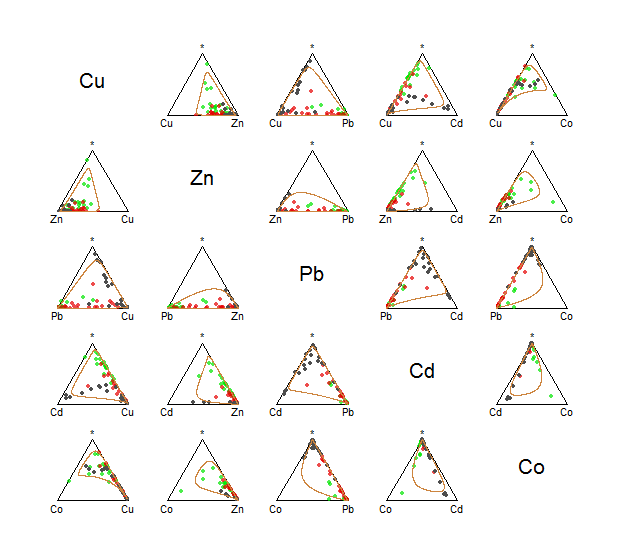
yielding only one curve per ternary diagram.enter image description here

in which the radius of the lines contain 95% of the probability assuming a normal model for the composition and a known variance.(minimally) paraphrasing:

in which the radius of the lines contain 95% of the probability assuming a normal model for the composition and a known variance.

... and there is a clarifying comment as to?ellipses describes the meaning of $*$r parameter in the function ellipses as:

margin = "acomp" (or nothing, the default) computes the third part as the geometric of all components except those two from row and colum (symbolized with "*").

r      a scaling of the half-diameters

What are the color-coded (black, redmeaning and green) lines on themathematics behind these deformed circles (firstlines or curves) plot? And, if at all possible - I understand this second part is code-specific - how can they be generated by the function ellipses?

So I've been trying to reproduce this matrix scatter plots, and understand them. For instance I am having trouble calling the multiple plots with the curves around points of the grouping categorical variable:

Here is my code and the output:

library(compositions)
data(SimulatedAmounts)
colors = c(rgb(red=0.3, green=0.3,  blue=.3, alpha=1),
           rgb(red=0.9, green=0,    blue=0, alpha=0.7),
           rgb(red=0,   green=.9,   blue=0, alpha=0.7))
           
tt = acomp(sa.groups5)
plot(tt, col = rgb(0,0,0,0), bg = colors[as.numeric(sa.groups.area)], pch = 21, cex = .9)
ellipses(mean(tt), var(tt), r = 2, col = "peru")

enter image description here

yielding only one curve per ternary diagram.

in which the radius of the lines contain 95% of the probability assuming a normal model for the composition and a known variance.

and there is a clarifying comment as to the meaning of $*$:

margin = "acomp" (or nothing, the default) computes the third part as the geometric of all components except those two from row and colum (symbolized with "*").

What are the color-coded (black, red and green) lines on the (first) plot? And, if at all possible - I understand this second part is code-specific - how can they be generated?

The "mystery" asterisk $(*)$ is clarified in this passage in Analyzing Compositional Data with R By K. Gerald van den Boogaart, Raimon Tolosana-Delgado

margin = "acomp" (or nothing, the default) computes the third part as the geometric of all components except those two from row and colum (symbolized with "*").


I've been trying to reproduce this matrix scatter plots, and understand them. For instance, I had trouble calling the multiple plots with the curves around points of the grouping categorical variable:

Finally, though, I got a practically identical plot with this code:

library(compositions)
data(SimulatedAmounts)
colors = c(rgb(red=0.3, green=0.3,  blue=.3, alpha=1),
           rgb(red=0.9, green=0,    blue=0, alpha=0.7),
           rgb(red=0,   green=.9,   blue=0, alpha=0.7))
           
tt = acomp(sa.groups5)
plot(tt, col = rgb(0,0,0,0), bg = colors[as.numeric(sa.groups.area)], pch = 21, cex = .9)
ellipses(mean(tt), var(tt), r = 2, col = "peru")

strata = sa.groups5.area
temp = cbind(sa.groups5,strata)

a = acomp(temp[temp[ , 6] == 1, ][,1:5])
ellipses(mean(a), var(a), r = 2, col = colors[1])

b = acomp(temp[temp[ , 6] == 2, ][,1:5])
ellipses(mean(b), var(b), r = 2, col = colors[2])

c = acomp(temp[temp[ , 6] == 3, ][,1:5])
ellipses(mean(c), var(c), r = 2, col = colors[3])

enter image description here

and (minimally) paraphrasing:

in which the radius of the lines contain 95% of the probability assuming a normal model for the composition and a known variance.

... and ?ellipses describes the r parameter in the function ellipses as:

r      a scaling of the half-diameters

What are the meaning and mathematics behind these deformed circles (lines or curves) generated by the function ellipses?

added 141 characters in body
Source Link
Antoni Parellada
  • 26.9k
  • 18
  • 122
  • 230
Loading
deleted 17 characters in body
Source Link
Antoni Parellada
  • 26.9k
  • 18
  • 122
  • 230
Loading
edited body
Source Link
Antoni Parellada
  • 26.9k
  • 18
  • 122
  • 230
Loading
added 14 characters in body
Source Link
Antoni Parellada
  • 26.9k
  • 18
  • 122
  • 230
Loading
edited title
Link
Antoni Parellada
  • 26.9k
  • 18
  • 122
  • 230
Loading
added 1 character in body; edited title
Source Link
Antoni Parellada
  • 26.9k
  • 18
  • 122
  • 230
Loading
added 2 characters in body
Source Link
Antoni Parellada
  • 26.9k
  • 18
  • 122
  • 230
Loading
deleted 134 characters in body
Source Link
Antoni Parellada
  • 26.9k
  • 18
  • 122
  • 230
Loading
added 633 characters in body
Source Link
Antoni Parellada
  • 26.9k
  • 18
  • 122
  • 230
Loading
added 363 characters in body
Source Link
Antoni Parellada
  • 26.9k
  • 18
  • 122
  • 230
Loading
added 42 characters in body
Source Link
Antoni Parellada
  • 26.9k
  • 18
  • 122
  • 230
Loading
Source Link
Antoni Parellada
  • 26.9k
  • 18
  • 122
  • 230
Loading