Why is the formula for standard error the way it is?

Question

So just "why" is $SE = \frac{s}{\sqrt n}$ ? How should one interpret/articulate the reason of having $\sqrt n$ in the denominator. Why do we divide sample mean by the square root of the sample size, intuitively speaking? And how/why is it called standard "error". (Question equally applicable for true standard deviation of the population: $\frac{\sigma}{\sqrt n}$)

Is there an intuitive derivation of $SE$ that can make this clear?

Please assume you are explaining it to a 6 year old who understands mean and sample size :)

Answer 1

This comes from the fact that $\newcommand{\Var}{\operatorname{Var}}\newcommand{\Cov}{\operatorname{Cov}}\Var(X+Y) = \Var(X) + \Var(Y) + 2\cdot\Cov(X,Y)$ and for a constant $a$, $\Var( a X ) = a^2 \Var(X)$.

Since we are assuming that the individual observations are independent the $\Cov(X,Y)$ term is $0$ and since we assume that the observations are identically distributed all the variances are $\sigma^2$. So

$\Var( \frac{1}{n} \sum X_i ) = \frac{1}{n^2} \sum \Var(X_i) = \frac{1}{n^2} \times \sum_{i=1}^n \sigma^2= \frac{n}{n^2} \sigma^2 = \frac{\sigma^2}{n}$

And when we take the square root of that (because it is harder to think on the variance scale) we get $\dfrac{\sigma}{\sqrt{n}}$.

More intuitively, think of 2 statistics classes: in the first the teacher assigns each of the students to draw a sample of size 10 from a set of tiles with numbers on them (the teacher knows the true mean of this population, but the students don't) and compute the mean of their sample. The second teacher assigns each of his/her students to take samples of size 100 from the same set of tiles and compute the mean. Would you expect every sample mean to exactly match the population mean? or to vary about it? Would you expect the spread of the sample means to be the same in both classes? or would the 2nd class tend to be closer to the population? That's why it makes sense to divide by a function of the sample size. The square root means we have a law of diminishing returns, to halve the standard error you need to quadruple the sample size.

As for the name, the full name is "The estimated standard deviation of the sampling distribution of x-bar"; it only takes saying that a few times before you appreciate having a shortened form. I don't know who first substituted "error" for "deviation" this way, but it stuck. The standard deviation measures variability of individual observations; the standard error measures variability in estimates of parameters (based on observations).

Answer 2

Why √n?

So there is this theory called the central limit theorem that tells us that as sample size increases, sampling distributions of means become normally distributed regardless of the parent distribution. In other words, given a sufficiently large sample size, the mean of all samples from a population will be the same as the population mean. We know that this really happens. Let’s put that in the bank and revisit it later.

Now, let's look at what happens when we have a small sample size (n=5), and then observe what happens if we increase the sample size and leave all the population parameters the same.

population mean: 15 standard deviation: 5 N=5

In the above case, our standard error of the mean (S.E.M.) will be: 5/√5 = 2.236

Now let's consider a case with a sample size of 10

population mean: 15 standard deviation: 5 N=10

S.E.M. will be: 5/√10 = 1.158

Increase the sample to 100: S.E.M = 5/√100 = .5

Increase the sample to 1000: S.E.M = 5/√1000 = .158

...You see the pattern. As sample size increases, the standard error of the mean decreases and will continue to approach zero as your sample size increases infinitely. Why is this? One way to think about it is that if you keep increasing your sample size, you will eventually sample the entire population, at which point, your sample mean is your population mean. That is, any given sample mean will probably not be exactly equal to the true population mean, but as your sample size increases toward the size of the entire population, the amount that a given sample mean is likely to be off by (the standard error) becomes smaller and smaller.

Now, let's go back to the conceptual definition of the standard error of the mean. One way to look at it is as the "standard deviation of sample means", or, alternatively, "On average, a sample of size N will deviate from the population mean by this amount". Therefore, your S.E.M. statistic is giving you an idea of how well your sample mean is likely to approximate the population mean.

So we know that the S.E.M. tells us how well a sample mean of size N approximates the population mean, and we also know that as our sample size increases, any given sample mean will more closely approximate the population mean.

The mathematical expression of those two ideas is the formula for S.E.M.

By dividing by the square root of N, you are paying a “penalty” for using a sample instead of the entire population (sampling allows us to make guesses, or inferences, about a population. The smaller the sample, the less confidence you might have in those inferences; that’s the origin of the “penalty”). That penalty is relatively large when your sample is very small. As the sample size increases, however, that penalty rapidly diminishes, infinitely approaching the point where your sample is equivalent to the population itself.

How fast does a sample mean approach equivalence with the population mean (i.e., how fast does the S.E.M. approach 0) as the sample size increases? That will depend on the numerator in the formula: standard deviation. The standard deviation is a measure of how predictable any given observation is in a population, or how far from the mean any one observation is likely to be. The less predictability, the higher the standard deviation. By the same token, the higher the standard deviation, the less quickly your sample mean will approach the population mean as sample size N increases. The power of the central limit theorem, however, shows us that as sample sizes become very large, the S.E.M. becomes very small, regardless of the standard deviation. That is, having a sufficiently large sample size will lead to a very small S.E.M. in just about all cases. The main differences in this trend between large or small standard deviations appears most notably when sample sizes are small – you pay a large penalty for having a small sample from a population that has a lot of variability!

Answer 3

To answer this question, let's imagine you are doing an experiment. Maybe to measure the weight of a ball. Let's assume we don't know the true/precise weight of the ball. Of course, your measurement device and conditions are not perfect and it has some errors due to various reasons. So, you performed 5 experiments and you got these values - 1 kg, 1.1 kg, 0.9 kg, 0.94 kg, and 1.01 kg. Now, what does standard deviation tell you? It tells you how scattered your measurements are. Assuming these experiments are normally distributed around true weight (can be 1 kg in our case), standard deviation tells us the expected error in your single measurement.

Now suppose you want to reduce error in your measured weight. But, you can not change your measuring device or improve your measurement conditions. So, what's the solution? The solution is you can take the average of your individual experiments. Since, your measurement errors are normally distributed around the true weight, the positive and negative errors will cancel out if you take the average and the average of all 5 measurements will be more precise than any individual experiment. But the question is can you quantify the approximate difference between the average of your 5 values and the true weight? The answer is yes and this is what your standard error gives.

So, what if you are not satisfied with the precision of measurement that you get by taking the average over 5 experiments and you want to further improve the precision. In that case, you can perform 5 more experiments. Now, if you take average over these 10 experiments, your average measured weight will be closer to the true weight than the average of 5 experiments. It's intuitive that if you continue increasing the number of individual experiments, your precision will continue to increase.

But wait. What about your return on investment/efforts? Indeed conducting an experiment is not an easy task. It requires your manual efforts. If you move from 1 experiment to the average of 5 experiments, you are able to improve precision by say 10%. Then if you add 5 more experiments, your precision will not increase by 10% but somewhat less than that. and if you add 5 more in addition to the previous one, your increase in precision will be further lesser. and so on. Now the question is can you quantify the decrease in return on investment?

The answer is yes. The precision is approximately proportional to the square root of the number of experiments.

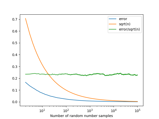
Let's see it graphically with a Python experiment. Let's sample 100000 random values between 0 to 1. Ideally, if these random values are distributed uniformly between 0 and 1, the expected value of the mean is 0.5. For finite sample sizes, there will be a finite difference (let's call it 'error') in the mean of the sample and the expected value of 0.5. This error should decrease as we increase the sample size. If we plot this error, against the sample size, it will look like the blue line in the following graph (Note: here this error is averaged over many experiments to reduce the fluctuations). Compare it with the square root of the number of experiments shown in orange color. We can see that both of them have similar shapes. In fact, if we plot the ratio of error and sqrt(n), it is a constant (shown with the green line). Woww!! That means the error in the measured mean indeed decreases as square root of the number of experiments. That's what the standard error formula told us. Interestingly, if you do some other experiment, the ratio might change, but the error will still be proportional to 1/sqrt(n).

Hope, now you have an intuition of standard error and the sqrt(n) in it.

The code to generate the above picture is this:

import numpy as np
from matplotlib import pyplot as plt

def plot(err, b=0,c='max'):
    n = len(err)
    if(type(c)==str):
        if(c=='max'):
            c = n
            
    x = np.arange(1,n+1)
    sqrtn = 1/np.sqrt(np.arange(1,n+1))
    
    plt.plot(x[b:c], err[b:c], label='error')
    plt.plot(x[b:c], sqrtn[b:c], label='sqrt(n)')
    ratio = err/sqrtn
    plt.plot(x[b:c], ratio[b:c], label='error/sqrt(n)')
    plt.xlabel('Number of random number samples')
    plt.legend(loc='best')
    plt.show()

def calc_err(n, seed=777001):
    np.random.seed(seed=seed)
    cum_n = np.arange(1,n+1)
    x = np.random.rand(n)
    cumsum = np.cumsum(x)
    cummean = cumsum/cum_n
    mu = 0.5#x.mean()
    #print(mu)
    err = np.absolute(cummean-mu)
    return err

n  = 100000
seed = 77701
seed_count = 1000

err_sum = np.zeros(n)
for seed in range(77700, 77700+seed_count):
    err = calc_err(n, seed)
    err_sum = err_sum+err
    
err = err_sum/seed_count   
plot(err, b=1, c='max')