Effect of switching response and explanatory variable in simple linear regression

Question

Let's say that there exists some "true" relationship between $y$ and $x$ such that $y = ax + b + \epsilon$, where $a$ and $b$ are constants and $\epsilon$ is i.i.d normal noise. When I randomly generate data from that R code: x <- 1:100; y <- ax + b + rnorm(length(x)) and then fit a model like y ~ x, I obviously get reasonably good estimates for $a$ and $b$.

If I switch the role of the variables as in (x ~ y), however, and then rewrite the result for $y$ to be a function of $x$, the resulting slope is always steeper (either more negative or more positive) than that estimated by the y ~ x regression. I'm trying to understand exactly why that is and would appreciate it if anyone could give me an intuition as to what's going on there.

Answer 1

Given $n$ data points $(x_i,y_i), i = 1,2,\ldots n$, in the plane, let us draw a straight line $y = ax+b$. If we predict $ax_i+b$ as the value $\hat{y}_i$ of $y_i$, then the error is $(y_i-\hat{y}_i) = (y_i-ax_i-b)$, the squared error is $(y_i-ax_i-b)^2$, and the total squared error $\sum_{i=1}^n (y_i-ax_i-b)^2$. We ask

What choice of $a$ and $b$ minimizes $S =\displaystyle\sum_{i=1}^n (y_i-ax_i-b)^2$?

Since $(y_i-ax_i-b)$ is the vertical distance of $(x_i,y_i)$ from the straight line, we are asking for the line such that the sum of the squares of the vertical distances of the points from the line is as small as possible. Now $S$ is a quadratic function of both $a$ and $b$ and attains its minimum value when $a$ and $b$ are such that $$\begin{align*} \frac{\partial S}{\partial a} &= 2\sum_{i=1}^n (y_i-ax_i-b)(-x_i) &= 0\\ \frac{\partial S}{\partial b} &= 2\sum_{i=1}^n (y_i-ax_i-b)(-1) &= 0 \end{align*}$$ From the second equation, we get $$b = \frac{1}{n}\sum_{i=1}^n (y_i - ax_i) = \mu_y - a\mu_x$$ where $\displaystyle \mu_y = \frac{1}{n}\sum_{i=1}^n y_i, ~ \mu_x = \frac{1}{n}\sum_{i=1}^n x_i$ are the arithmetic average values of the $y_i$'s and the $x_i$'s respectively. Substituting into the first equation, we get $$ a = \frac{\left(\frac{1}{n}\sum_{i=1}^n x_iy_i\right) -\mu_x\mu_y}{ \left( \frac{1}{n}\sum_{i=1}^n x_i^2\right) -\mu_x^2}. $$ Thus, the line that minimizes $S$ can be expressed as $$y = ax+b = \mu_y + \left(\frac{\left(\frac{1}{n}\sum_{i=1}^n x_iy_i\right) -\mu_x\mu_y}{ \left( \frac{1}{n}\sum_{i=1}^n x_i^2\right) -\mu_x^2}\right) (x - \mu_x), $$ and the minimum value of $S$ is $$S_{\min} = \frac{\left[\left(\frac{1}{n}\sum_{i=1}^n y_i^2\right) -\mu_y^2\right] \left[\left(\frac{1}{n}\sum_{i=1}^n x_i^2\right) -\mu_x^2\right] - \left[\left(\frac{1}{n}\sum_{i=1}^n x_iy_i\right) -\mu_x\mu_y\right]^2}{\left(\frac{1}{n}\sum_{i=1}^n x_i^2\right) -\mu_x^2}.$$

If we interchange the roles of $x$ and $y$, draw a line $x = \hat{a}y + \hat{b}$, and ask for the values of $\hat{a}$ and $\hat{b}$ that minimize $$T = \sum_{i=1}^n (x_i - \hat{a}y_i - \hat{b})^2,$$ that is, we want the line such that the sum of the squares of the horizontal distances of the points from the line is as small as possible, then we get

$$x = \hat{a}y+\hat{b} = \mu_x + \left(\frac{\left(\frac{1}{n}\sum_{i=1}^n x_iy_i\right) -\mu_x\mu_y}{ \left( \frac{1}{n}\sum_{i=1}^n y_i^2\right) -\mu_y^2}\right) (y - \mu_y) $$ and the minimum value of $T$ is $$T_{\min} = \frac{\left[\left(\frac{1}{n}\sum_{i=1}^n y_i^2\right) -\mu_y^2\right] \left[\left(\frac{1}{n}\sum_{i=1}^n x_i^2\right) -\mu_x^2\right] - \left[\left(\frac{1}{n}\sum_{i=1}^n x_iy_i\right) -\mu_x\mu_y\right]^2}{\left(\frac{1}{n}\sum_{i=1}^n y_i^2\right) -\mu_y^2}.$$

Note that both lines pass through the point $(\mu_x,\mu_y)$ but the slopes are $$a = \frac{\left(\frac{1}{n}\sum_{i=1}^n x_iy_i\right) -\mu_x\mu_y}{ \left( \frac{1}{n}\sum_{i=1}^n x_i^2\right) -\mu_x^2},~~ \hat{a}^{-1} = \frac{ \left( \frac{1}{n}\sum_{i=1}^n y_i^2\right) -\mu_y^2}{\left(\frac{1}{n}\sum_{i=1}^n x_iy_i\right) -\mu_x\mu_y}$$ are different in general. Indeed, as @whuber points out in a comment, the slopes are the same when all the points $(x_i,y_i)$ lie on the same straight line. To see this, note that $$\hat{a}^{-1} - a = \frac{S_{\min}}{\left(\frac{1}{n}\sum_{i=1}^n x_iy_i\right) -\mu_x\mu_y} = 0 \Rightarrow S_{\min} = 0 \Rightarrow y_i=ax_i+b, i=1,2,\ldots, n. $$

Answer 2

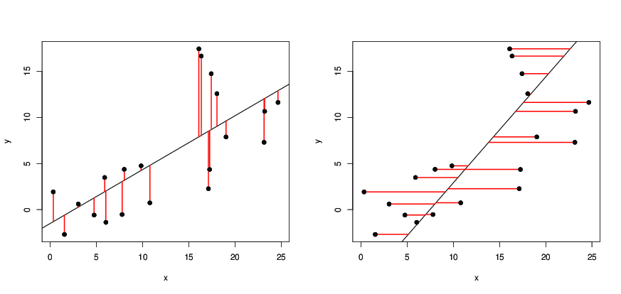
Just to illustrate Dilip’s answer: on the following pictures,

• the black dots are data points ;
• on the left, the black line is the regression line obtained by y ~ x, which minimize the squares of the length of the red segments;
• on the right, the black line is the regression line obtained by x ~ y, which minimize the squares of the length of the red segments.

Edit (least rectangles regression)

If there is no natural way to chose a "response" and a "covariate", but rather the two variables are interdependent you may wish to conserve a symmetrical role for $y$ and $x$; in this case you can use "least rectangles regression."

• write $Y = aX + b + \epsilon$, as usual;
• denote $\hat y_i = a x_i + b$ and $\hat x_i = {1\over a} (y_i - b)$ the estimations of $Y_i$ conditional to $X = x_i$ and of $X_i$ conditional to $Y = y_i$;
• minimize $\sum_i | x_i - \hat x_i | \cdot | y_i - \hat y_i|$, which leads to $$\hat y = \mathrm{sign}\left(\mathrm{cov}(x,y)\right){\hat\sigma_y \over \hat\sigma_x} (x-\overline x) + \overline y. $$

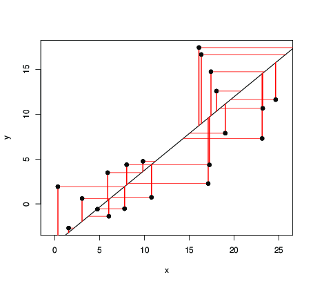
Here is an illustration with the same data points, for each point, a "rectangle" is computed as the product of the length of two red segments, and the sum of rectangles is minimized. I don’t know much about the properties of this regression and I don’t find much with google.

Answer 3

Just a brief note on why you see the slope smaller for one regression. Both slopes depend on three numbers: standard deviations of $x$ and $y$ ($s_{x}$ and $s_{y}$), and correlation between $x$ and $y$ ($r$). The regression with $y$ as response has slope $r\frac{s_{y}}{s_{x}}$ and the regression with $x$ as response has slope $r\frac{s_{x}}{s_{y}}$, hence the ratio of the first slope to the reciprocal of the second is equal to $r^2\leq 1$.

So the greater the proportion of variance explained, the closer the slopes obtained from each case. Note that the proportion of variance explained is symmetric and equal to the squared correlation in simple linear regression.

Answer 4

Regression line is not (always) the same as true relationship

You may have some 'true' causal relationship with an equation in a linear form $a+bx$ like

$$y := a + bx + \epsilon$$

Where the $:=$ means that the value of $a+bx$ with some added noise $\epsilon$ is assigned to $y$.

The fitted regression lines y ~ x or x ~ y do not mean the same as that causal relationship (even when in practice the expression for one of the regression line may coincide with the expression for the causal 'true' relationship)

---

More precise relationship between slopes

For two switched simple linear regressions:

$$Y = a_1 + b_1 X\\X = a_2 + b_2 Y$$

you can relate the slopes as following:

$$b_1 = \rho^2 \frac{1}{b_2} \leq \frac{1}{b_2}$$

So the slopes are not each other inverse.

---

Intuition

The reason is that

• Regression lines and correlations do not necessarily correspond one-to-one to a causal relationship.
• Regression lines relate more directly to a conditional probability or best prediction.

You can imagine that the conditional probability relates to the strength of the relationship. Regression lines reflect this and the slopes of the lines may be both shallow when the strength of the relationship is small or both steep when the strength of the relationship is strong. The slopes are not simply each others inverse.

Example

If two variables $X$ and $Y$ relate to each other by some (causal) linear relationship $$Y = \text{a little bit of $X + $ a lot of error}$$ Then you can imagine that it would not be good to entirely reverse that relationship in case you wish to express $X$ based on a given value of $Y$.

Instead of

$$X = \text{a lot of $Y + $ a little of error}$$

it would be better to also use

$$X = \text{a little bit of $Y + $ a lot of error}$$

See the following example distributions with their respective regression lines. The distributions are multivariate normal with $\Sigma_{11} \Sigma_{22}=1$ and $\Sigma_{12} = \Sigma_{21} = \rho$

The conditional expected values (what you would get in a linear regression) are

$$\begin{array}{} E(Y|X) &=& \rho X \\ E(X|Y) &=& \rho Y \end{array}$$

and in this case with $X,Y$ a multivariate normal distribution, then the conditional distributions are

$$\begin{array}{} Y|X & \sim & N(\rho X,1-\rho^2) \\ X|Y & \sim & N(\rho Y,1-\rho^2) \end{array}$$

So you can see the variable Y as being a part $\rho X$ and a part noise with variance $1-\rho^2$. The same is true the other way around.

The larger the correlation coefficient $\rho$, the closer the two lines will be. But the lower the correlation, the less strong the relationship, the less steep the lines will be (this is true for both lines Y ~ X and X ~ Y)

Answer 5

A simple way to look at this is to note that, if for the true model $y=\alpha+\beta x+\epsilon$, you run two regressions:

• $y=a_{y\sim x}+b_{y\sim x} x$
• $x=a_{x\sim y}+b_{x\sim y} y$

Then we have, using $b_{y\sim x}=\frac{cov(x,y)}{var(x)}=\frac{cov(x,y)}{var(y)}\frac{var(y)}{var(x)}$:

$$b_{y\sim x}=b_{x\sim y}\frac{var(y)}{var(x)}$$

So whether you get a steeper slope or not just depends on the ratio $\frac{var(y)}{var(x)}$. This ratio is equal to, based on the assumed true model:

$$\frac{var(y)}{var(x)}=\frac{\beta^2 var(x) + var(\epsilon)}{var(x)}$$

Link with other answers

You can connect this result with the answers from others, who said that when $R^2=1$, it should be the reciprocal. Indeed, $R^2=1\Rightarrow var(\epsilon) = 0$, and also, $b_{y\sim x}=\beta$ (no estimation error), Hence:

$$R^2=1\Rightarrow b_{y\sim x}=b_{x\sim y}\frac{\beta^2 var(x) + 0}{var(x)}=b_{x\sim y}\beta^2$$

So $b_{x\sim y}=1/\beta$

Answer 6

It becomes interesting when there is also noise on your inputs (which we could argue is always the case, no command or observation is ever perfect).

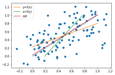
I have built some simulations to observe the phenomenon, based on a simple linear relationship $x = y$, with Gaussian noise on both x and y. I generated the observations as follows (python code):

x = np.linspace(0, 1, n)
y = x

x_o = x + np.random.normal(0, 0.2, n)
y_o = y + np.random.normal(0, 0.2, n)

See the different results (odr here is orthogonal distance regression, i.e. the same as least rectangles regression):

All the code is in there:

https://gist.github.com/jclevesque/5273ad9077d9ea93994f6d96c20b0ddd

Answer 7

The short answer

The goal of a simple linear regression is to come up with the best predictions of the y variable, given values of the x variable. This is a different goal than trying to come up with the best prediction of the x variable, given values of the y variable.

Simple linear regression of y ~ x gives you the 'best' possible model for predicting y given x. Hence, if you fit a model for x ~ y and algebraically inverted it, that model could at its very best do only as well as the model for y ~ x. But inverting a model fit for x ~ y will usually do worse at predicting y given x, compared to the 'optimal' y ~ x model, because the "inverted x ~ y model" was created to fulfill a different objective.

Illustration

Imagine you have the following dataset:

When you run an OLS regression of y ~ x, you come up with the following model

y = 0.167 + 1.5*x

This optimizes predictions of y by making the following predictions, which have associated errors:

The OLS regression's predictions are optimal in the sense that the sum of the values in the rightmost column (i.e. the sum of squares) is as small as can be.

When you run an OLS regression of x ~ y, you come up with a different model:

x = -0.07 + 0.64*y

This optimizes predictions of x by making the following predictions, with associated errors.

Again, this is optimal in the sense that the sum of the values of the rightmost column are as small as possible (equal to 0.071).

Now, imagine you tried to just invert the first model, y = 0.167 + 1.5*x, using algebra, giving you the model x = -0.11 + 0.67*x.

This would give you the following predictions and associated errors:

The sum of the values in the rightmost column is 0.074, which is larger than the corresponding sum from the model you get from regressing x on y, i.e. the x ~ y model. In other words, the "inverted y ~ x model" is doing a worse job at predicting x than the OLS model of x ~ y.

Answer 8

One useful fact about the residuals of the OLS Y ~ X and the X ~ Y regressions is that their correlation is then opposite of the correlation between Y and X.

Write Y = a1 + b1 X + e1 and X = a2 + b2 Y + e2.

If we denote r=corr(X,Y) the OLS estimates are

b1 = r * sY / sX

and

b2 = r * sX / sY

where sX is the standard deviation of X and sY the standard deviation of Y.

Then

Cov(e1,e2) = - r (1-r^2) sX sY, Var(e1) = sY^2 (1-r^2), Var(e2) = sX^2 (1-r^2),

so Cor(e1,e2)= -r!