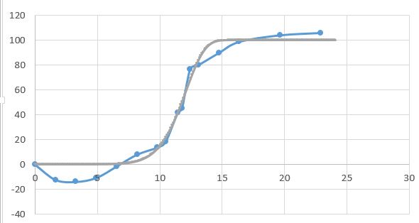
To fit a sigmoid-like function in a nonparametric way, we could use a monotone spline. This is implemented in the R package (all R packages here referenced are on CRAN) splines2. I will borrow some R code from the answer by @Chaconne, and modify it for my needs.
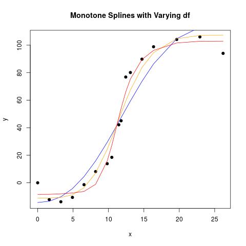
splines2 offers the functions mSpline, implementing M-splines, which is a everywhere nonnegative (on the interval where defined) spline basis, and iSpline, the integral of the M-spline basis. The last one then are monotone increasing, so we can fit an increasing function by using them as a regression spline basis, and fit a linear model with restrictions on the coefficients to be non-negative. The last is implemented in a user-friendly way by R package colf, "constrained optimization on linear functions". The fits look like:

The R code used:
library(splines2) # includes monotone splines,  M-splines,  I-splines.
library(colf) # constrained optimization on linear functions

 txt <- "| 0             | 0              |
    | 1.6366666667  | -12.2012787905 |
    | 3.2733333333  | -13.7833876716 |
    | 4.91          | -10.5943208589 |
    | 6.5466666667  | -1.3584575518  |
    | 8.1833333333  | 8.1590423167   |
    | 9.82          | 13.8827937482  |
    | 10.4746666667 | 18.4965880076  |
    | 11.4566666667 | 42.1205206106  |
    | 11.784        | 45.0528073182  |
    | 12.4386666667 | 76.8150755186  |
    | 13.0933333333 | 80.0883540997  |
    | 14.73         | 89.7784173678  |
    | 16.3666666667 | 98.8113459392  |
    | 19.64         | 104.104366506  |
    | 22.9133333333 | 105.9929585305 |
    | 26.1866666667 | 94.0070414695  |"

    dat <- read.table(text=txt, sep="|")[,2:3]
names(dat) <- c("x", "y")
plot(dat$y ~ dat$x, pch = 19, xlab = "x", ylab = "y", main = "Monotone Splines with Varying df")

Imod_df_4  <-  colf_nls(y ~ 1 + iSpline(x, df=4), data=dat, lower=c(-Inf, rep(0, 4)), control=nls.control(maxiter=1000, tol=1e-09, minFactor=1/2048) )
lines(dat$x, fitted(Imod_df_4), col="blue")

Imod_df_6  <-  colf_nls(y ~ 1 + iSpline(x, df=6), data=dat, lower=c(-Inf, rep(0, 6)), control=nls.control(maxiter=1000, tol=1e-09, minFactor=1/2048) )
lines(dat$x, fitted(Imod_df_6), col="orange")

Imod_df_8  <-  colf_nls(y ~ 1 + iSpline(x, df=8), data=dat, lower=c(-Inf, rep(0, 8)), control=nls.control(maxiter=1000, tol=1e-09, minFactor=1/2048) )
lines(dat$x, fitted(Imod_df_8), col="red")

EDIT
Monotone restrictions on a spline is a special case of shape-restricted splines, and now there is one (in fact several) R packages implementing those simplifying their use. I will do the above example again, with one of those packages. The R code is below, using the data as read in above:
library(cgam)

mod_cgam0 <- cgam(y ~ 1+s.incr(x), data=dat, family=gaussian)
summary(mod_cgam0)
Call:
cgam(formula = y ~ 1 + s.incr(x), family = gaussian, data = dat)

Coefficients:
            Estimate  StdErr t.value   p.value
(Intercept)  43.4925  2.7748  15.674 < 2.2e-16 ***
---
Signif. codes:  0 ‘***’ 0.001 ‘**’ 0.01 ‘*’ 0.05 ‘.’ 0.1 ‘ ’ 1

(Dispersion parameter for gaussian family taken to be 102.2557)

Null deviance:  33749.25  on 16  degrees of freedom
Residual deviance:  1636.091  on 12.5  observed degrees of freedom

Approximate significance of smooth terms:
          edf mixture.of.Beta   p.value
s.incr(x)   3          0.9515 < 2.2e-16 ***
---
Signif. codes:  0 ‘***’ 0.001 ‘**’ 0.01 ‘*’ 0.05 ‘.’ 0.1 ‘ ’ 1
CIC:  7.6873
This way the knots (and degrees of freedom) has been selected automatically. To fix the number of degrees of freedom use:
mod_cgam1 <- cgam(y ~ 1+s.incr(x, numknots=5), data=dat, family=gaussian)
A paper presenting cgam is here (arxiv).

