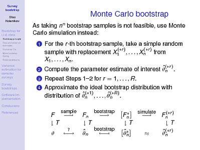
This is probably a more technical explanation aimed at people who understand some statistics and mathematics (calculus, at least). Here's a slide from a course on survey bootstraps that I taught some while ago:

Some explanations are needed, of course. $T$ is the procedure to obtain the statistic from the existing data (or, to be technically precise, a functional from the distribution function to real numbers; e.g., the mean is $E[X]=\int x {\rm d}F$, where for the sample distribution function $F_n()$, the ${\rm d}F$ is understood as a point mass at a sample point). In the population, denoted by $F()$, application of $T$ gives the parameter of interest $\theta$. Now, we've taken a sample (the first arrow on the top), and have the empirical distribution function $F_n()$ -- we apply $T$ to it to obtain the estimate $\hat\theta_n$. How far is it from $\theta$, we wonder? What is the distribution that the random quantity $\hat\theta_n$ may have around $\theta$? This is the question mark in the lower left of the diagram, and this is the question the bootstrap tries to answer. To restate gung's point, this is not the question about the population, but the question about a particular statistic and its distribution.
If we could repeat our sampling procedure, we could get that distribution and learn more. Well, that usually is beyond our capabilities. However, if
- $F_n$ is close enough to $F$, in a suitable sense, and
- the mapping $T$ is smooth enough, i.e., if we take small deviations from $F()$, the results will be mapped to numbers close to $\theta$,
we can hope that the bootstrap procedure will work. Namely, we pretend that our distribution is $F_n()$ rather than $F()$, and with that we can entertain all possible samples -- and there will be $n^n$ such samples, which is only practical for $n\le 5$. Let me repeat again: the bootstrap works to create the sampling distribution of $\hat\theta_n^*$ around the "true" parameter $\hat\theta_n$, and we hope that with the two above conditions, this sampling distribution is informative about the sampling distribution of $\hat\theta_n$ around $\theta$:
$$
\hat\theta_n^* \mbox{ to } \hat\theta_n \mbox{ is like } \hat\theta_n \mbox{ to } \theta
$$
Now, instead of just going one way along the arrows, and losing some information/accuracy along these arrows, we can go back and say something about variability of $\hat\theta_n^*$ around $\hat\theta_n$.
The above conditions are spelled out it utmost technicality in Hall's The Bootstrap and Edgeworth Expansion (1992) book. The understanding of calculus that I said may be required as a prerequisite to staring at this slide is the second assumption concerning smoothness: in more formal language, the functional $T$ must possess a weak derivative. The first condition is, of course, an asymptotic statement: the larger your sample, the closer $F_n$ should become to $F$; and the distances from $\hat\theta_n^*$ to $\hat
\theta_n$ should be the same order of magnitude as those from $\hat\theta_n$ to $\theta$. These conditions may break, and they do break (Canty et al 2006 CJS) in a number of practical situations with weird enough statistics and/or sampling schemes that do not produce empirical distributions that are close enough to $F$.
Now, where does that 1000 samples, or whatever the magic number might be, comes from? It comes from our inability to draw all $n^n$ samples, so we just take a random subset of these. The right most "simulate" arrow states another approximation that we are making on our way to get the distribution of $\hat\theta_n$ around $\theta$, and that is to say that our Monte Carlo simulated distribution of $\hat\theta_n^{(*r)}$ is a good enough approximation of the complete bootstrap distribution of $\hat\theta_n^*$ around $\hat\theta_n$.

