What measure of effect size in ANOVA has mode at zero under the null (unlike $\eta^2$ that does not)?

Question

I encountered a weird effect when computing eta squared in ANOVA. Here is a short simulation to demonstrate it.

I simulate $k$ groups with $n=10$ each, with all values drawn from standard normal distribution (i.e. under null hypothesis of no difference between groups). I conduct a one-way ANOVA to compare these groups, and compute eta squared $\eta^2 = \mathrm{SS}_\mathrm{btw}/\mathrm{SS}_\mathrm{tot}$ as a measure of effect size. I then plot the histogram of resulting values over many simulations. Here is the figure for $k=2,5,10$:

One can see that whereas at $k=2$ the distribution peaks at zero, with more groups the distribution starts to peak at a non-zero positive value. I have a number of questions about this phenomenon.

1. I did some googling (and searched this forum) and see that eta squared is often called a "biased" measure of effect size. Does this refer exactly to what I stumbled upon?

   Update: no. As @gung and @Silverfish clarified below, eta squared is trivially biased because it is constrained to be positive, and so $\mathbb{E}(\eta^2) \ne 0$ under the null, meaning that it is by definition biased. I am talking about a different phenomenon that does not seem to have a name (?), so I will call it "mode-biased-under-null".

2. Under what conditions does this mode-bias-under-null appear? I cannot get it with a t-test ($k=2$), both with equal and non-equal sample sizes, and seem to fail to get it with $k=3$. What is a condition (in terms of $k$ and $n_i$) that guarantees that the mode will be at zero?

   Update: it seems that the answer is $k \le 3$. Please see discussion here: What is the distribution of $R^2$ in linear regression under the null hypothesis? Why is its mode not at zero when $k>3$?

3. What are the alternatives to eta squared that do not suffer from this weird mode-biadness-under-null?

   I would like to have a measure of effect size (informally: measure of "separability" between groups) that:

   • is unbiased can be biased, but should peak at zero under the null hypothesis;
   • is between $0$ and $1$ so that $0$ can be interpreted as full overlap between groups and $1$ as non-overlapping distributions of groups (i.e. $100\%$ classification accuracy by a trivial algorithm);
   • does not have to be given by a simple formula, as long as it can be computed (e.g. for $k=2$ an area under a ROC curve would be an option);
   • works with unbalanced groups;
   • generalizes to n-way ANOVA with several factors, as eta squared generalizes to partial eta squared (but no nesting, repeated measures, or other nasty ANOVA designs are of interest to me; just e.g. two factors with an interaction).

---

Update: why would I care about it?

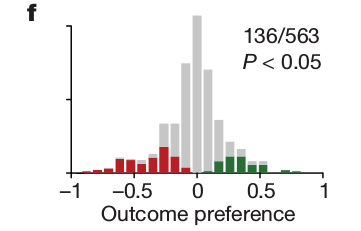
In my field (neuroscience) people often test a whole bunch of DVs (activity of single neurons) for dependency on some categorical IVs. Often this is done when there is only one categorical IV of interest, and it is binary. In this case, a histogram of effect sizes is often plotted across a population of neurons. Here is one example from this Nature paper:

Here $563$ neurons were tested, $136$ showed significant difference at $p<0.05$ level, and effect size ("outcome preference") was computed as an appropriately scaled area under the ROC curve.

I want to make a similar histogram, but when neurons are tested for tuning not to a binary factor, but to a multilevel factor. So I was going to run ANOVA and use $\eta^2$ as the effect size (or perhaps signed $\eta$, as my factor is in fact ordinal, so a meaningful sign can be attached to $\sqrt{\eta^2}$), but the resulting histogram does not peak at zero (and in case of signed $\eta$ it is bimodal), which will definitely confuse all the readers.

Answer 1

$\eta^2$ is the same as $R^2$ in a one-way ANOVA. It is bounded by $[0,\ 1]$. When the null hypothesis holds, the true value of $\eta^2$ is $0$. So the estimator $SSB/SST$ must be biased unless either it can only return $0$ when the null hypothesis is true, or if half its distribution is $<0$. Since it cannot be $<0$, and it can yield non-zero values, even when the null obtains, it must be biased. On the other hand, it is consistent, in the sense that $\eta^2\rightarrow 0$ as $N$ goes to infinity when the null holds.