95
$\begingroup$

Ridge regression coefficient estimate $\hat{\beta}^R$ are the values that minimize the

$$ \text{RSS} + \lambda \sum_{j=1}^p\beta_j^2. $$

My questions are:

  1. If $\lambda = 0$, then we see that the expression above reduces to the usual RSS. What if $\lambda \to \infty$? I do not understand the textbook explanation of the behaviour of the coefficients.

  2. To aid in understanding the concept behind a particular term, why is the term called RIDGE Regression? (Why ridge?) And what could have been wrong with the usual/common regression that there is a need to introduce a new concept called ridge regression?

Your insights would be great.

$\endgroup$

3 Answers 3

125
$\begingroup$

Since you ask for insights, I'm going to take a fairly intuitive approach rather than a more mathematical tack:

  1. Following the concepts in my answer here, we can formulate a ridge regression as a regression with dummy data by adding $p$ (in your formulation) observations, where $y_{n+j}=0$, $x_{j,n+j}=\sqrt{\lambda}$ and $x_{i,n+j}=0$ for $i\neq j$. If you write out the new RSS for this expanded data set, you'll see the additional observations each add a term of the form $(0-\sqrt{\lambda}\beta_j)^2=\lambda\beta_j^2$, so the new RSS is the original $\text{RSS} + \lambda \sum_{j=1}^p\beta_j^2$ -- and minimizing the RSS on this new, expanded data set is the same as minimizing the ridge regression criterion.

    So what can we see here? As $\lambda$ increases, the additional $x$-rows each have one component that increases, and so the influence of these points also increases. They pull the fitted hyperplane toward themselves. Then as $\lambda$ and the corresponding components of the $x$'s go off to infinity, all the involved coefficients "flatten out" to $0$.

    That is, as $\lambda\to\infty$, the penalty will dominate the minimization, so the $\beta$s will go to zero. If the intercept is not penalized (the usual case) then the model shrinks more and more toward the mean of the response.

  2. I'll give an intuitive sense of why we're talking about ridges first (which also suggests why it's needed), then tackle a little history. The first is adapted from my answer here:

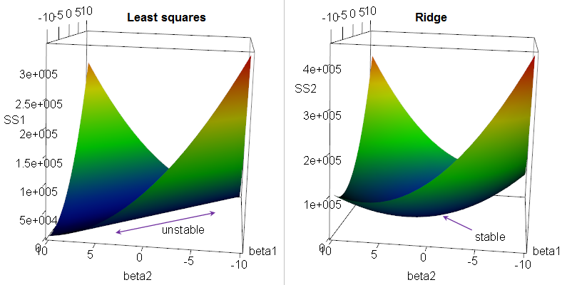
    If there's multicollinearity, you get a "ridge" in the likelihood function (likelihood is a function of the $\beta$'s). This in turn yields a long "valley" in the RSS (since RSS=$-2\log\mathcal{L}$).

    Ridge regression "fixes" the ridge - it adds a penalty that turns the ridge into a nice peak in likelihood space, equivalently a nice depression in the criterion we're minimizing:

    ridge in LS is turned into a peak in ridge regression
    [Clearer image]

    The actual story behind the name is a little more complicated. In 1959 A.E. Hoerl [1] introduced ridge analysis for response surface methodology, and it very soon [2] became adapted to dealing with multicollinearity in regression ('ridge regression'). See for example, the discussion by R.W. Hoerl in [3], where it describes Hoerl's (A.E. not R.W.) use of contour plots of the response surface* in the identification of where to head to find local optima (where one 'heads up the ridge'). In ill-conditioned problems, the issue of a very long ridge arises, and insights and methodology from ridge analysis are adapted to the related issue with the likelihood/RSS in regression, producing ridge regression.

* examples of response surface contour plots (in the case of quadratic response) can be seen here (Fig 3.9-3.12).

That is, "ridge" actually refers to the characteristics of the function we were attempting to optimize, rather than to adding a "ridge" (+ve diagonal) to the $X^TX$ matrix (so while ridge regression does add to the diagonal, that's not why we call it 'ridge' regression).

For some additional information on the need for ridge regression, see the first link under list item 2. above.


References:

[1]: Hoerl, A.E. (1959). Optimum solution of many variables equations. Chemical Engineering Progress, 55 (11) 69-78.

[2]: Hoerl, A.E. (1962). Applications of ridge analysis to regression problems. Chemical Engineering Progress, 58 (3) 54-59.

[3] Hoerl, R.W. (1985). Ridge Analysis 25 Years Later. American Statistician, 39 (3), 186-192

$\endgroup$
3
  • 2
    $\begingroup$ This is extremely helpful. Yes, when I was asking for insights, I was looking for intuition. Of course the mathematics is important, but I was also looking for conceptual explanations, because there are some parts when the math was just beyond me. Thanks again. $\endgroup$
    – cgo
    Commented May 8, 2015 at 12:03
  • $\begingroup$ Why do you have the word "weighted" in bullet point 1? $\endgroup$
    – amoeba
    Commented Apr 12, 2018 at 13:25
  • 2
    $\begingroup$ It's a good question; there's no need for it to be weighted unless the original regression was weighted. I have removed the adjective. It's also possible to write it as a weighted regression (which if you're already doing weighted regression might be very slightly easier to deal with). $\endgroup$
    – Glen_b
    Commented Apr 12, 2018 at 23:17
39
$\begingroup$
  1. If $\lambda \rightarrow \infty$ then our penalty term will be infinite for any $\beta$ other than $\beta = 0$, so that's the one we'll get. There is no other vector that will give us a finite value of the objective function.

(Update: Please see Glen_b's answer. This is not the correct historical reason!)

  1. This comes from ridge regression's solution in matrix notation. The solution turns out to be $$ \hat \beta = (X^TX + \lambda I)^{-1} X^TY. $$ The $\lambda I$ term adds a "ridge" to the main diagonal and guarantees that the resulting matrix is invertible. This means that, unlike OLS, we'll always get a solution.

Ridge regression is useful when the predictors are correlated. In this case OLS can give wild results with huge coefficients, but if they are penalized we can get much more reasonable results. In general a big advantage to ridge regression is that the solution always exists, as mentioned above. This applies even to the case where $n < p$, for which OLS cannot provide a (unique) solution.

Ridge regression also is the result when a normal prior is put on the $\beta$ vector.

Here's the Bayesian take on ridge regression: Suppose our prior for $\beta$ is $\beta \sim N(0, \frac{\sigma^2}{\lambda}I_p)$. Then because $(Y|X, \beta) \sim N(X\beta, \sigma^2 I_n)$ [by assumption] we have that $$ \pi(\beta | y) \propto \pi(\beta) f(y|\beta) $$

$$ \propto \frac{1}{(\sigma^2/\lambda)^{p/2}} \exp \left( -{\lambda \over 2\sigma^2} \beta^T\beta \right) \times \frac{1}{(\sigma^2)^{n/2}} \exp \left( \frac{-1}{2\sigma^2} ||y - X\beta||^2 \right) $$

$$ \propto \exp \left( -{\lambda \over 2\sigma^2} \beta^T\beta - \frac{1}{2\sigma^2} ||y - X\beta||^2 \right). $$

Let's find the posterior mode (we could look at posterior mean or other things too but for this let's look at the mode, i.e. the most probable value). This means we want $$ \max_{\beta \in \mathbb R^p} \ \exp \left( -{\lambda \over 2\sigma^2} \beta^T\beta - \frac{1}{2\sigma^2} ||y - X\beta||^2 \right) $$ which is equivalent to

$$ \max_{\beta \in \mathbb R^p} \ -{\lambda \over 2\sigma^2} \beta^T\beta - \frac{1}{2\sigma^2} ||y - X\beta||^2 $$ because $\log$ is strictly monotone and this in turn is equivalent to $$ \min_{\beta \in \mathbb R^p} ||y - X\beta||^2 + \lambda \beta^T\beta $$

which ought to look pretty familiar.

Thus we see that if we put a normal prior with mean 0 and variance $\frac{\sigma^2}{\lambda}$ on our $\beta$ vector, the value of $\beta$ which maximizes the posterior is the ridge estimator. Note that this treats $\sigma^2$ more as a frequentist parameter because there's no prior on it but it isn't known, so this isn't fully Bayesian.

Edit: you asked about the case where $n < p$. We know that a hyperplane in $\mathbb R^p$ is defined by exactly $p$ points. If we are running a linear regression and $n = p$ then we exactly interpolate our data and get $||y - X\hat\beta||^2 = 0$. This is a solution, but it is a terrible one: our performance on future data will most likely be abysmal. Now suppose $n < p$: there is no longer a unique hyperplane defined by these points. We can fit a multitude of hyperplanes, each with 0 residual sum of squares.

A very simple example: suppose $n = p = 2$. Then we'll just get a line between these two points. Now suppose $n = 2$ but $p = 3$. Picture a plane with these two points in it. We can rotate this plane without changing the fact that these two points are in it, so there are uncountably many models all with a perfect value of our objective function, so even beyond the issue of overfitting it is not clear which one to pick.

As a final comment (per @gung's suggestion), the LASSO (using an $L_1$ penalty) is commonly used for high dimensional problems because it automatically performs variable selection (sets some $\beta_j = 0$). Delightfully enough, it turns out that the LASSO is equivalent to finding the posterior mode when using a double exponential (aka Laplace) prior on the $\beta$ vector. The LASSO also has some limitations, such as saturating at $n$ predictors and not necessarily handling groups of correlated predictors in an ideal fashion, so the elastic net (convex combination of $L_1$ and $L_2$ penalties) may be brought to bear.

$\endgroup$
3
  • $\begingroup$ I appreciate your response. Thank you. Just another question though, I do not follow the statement: 'this applies even to the case when $n<p$...'. $p$ is the number of predictors, and $n$ is the number of samples right? What happens when $n<p$? Please give a very basic example why OLS can't give a unique solution. $\endgroup$
    – cgo
    Commented May 7, 2015 at 19:22
  • 4
    $\begingroup$ OLS can't find a unique solution when $n<p$ because the design matrix is not full rank. This is a very common question; please search the archives for a description of why this doesn't work. $\endgroup$
    – Sycorax
    Commented May 7, 2015 at 19:31
  • 2
    $\begingroup$ @cgo: user777's explanation and suggestion to search about is a good one, but for the sake of completeness I've also added a (hopefully) intuitive explanation. $\endgroup$
    – jld
    Commented May 7, 2015 at 19:43
0
$\begingroup$

why is the term called Ridge Regression?

From Ridge Regression: Biased Estimation for Nonorthogonal Problems (1970):

A. E. Hoerl first suggested in 1962 [9] [11] that to control the inflation and general instability associated with the least squares estimates, one can use

$$\beta^* = [X'X + kI]^{-1}X'Y; k \geq 0 (2.1) \\\\ = WX'Y (2.2)$$

The family of estimates given by $k \geq 0$ has many mathematical similarities with the portrayal of quadratic response functions [10]. For this reason, estimation and analysis built around (2.1) has been labeled "ridge regression."

$\endgroup$
1
  • 1
    $\begingroup$ This is historically correct, but it doesn't quite get to the answer: the reason for this term lies in the fact that Ridge Regression was conceptualized as (1) being applied to the negative of the objective function (that is, as a maximization problem) and (2) being used when the original quadratic (for $k=0$) is degenerate or very nearly so. The simplest non-trivial case of this situation is exemplified by the equation $z = -y^2$ whose graph in $(x,y,z)$ coordinates indeed looks like an anticline or "ridge" of a mountain chain. @ glen_b's answer explains and illustrates the second point. $\endgroup$
    – whuber
    Commented Nov 24, 2020 at 15:41

Your Answer

By clicking “Post Your Answer”, you agree to our terms of service and acknowledge you have read our privacy policy.

Not the answer you're looking for? Browse other questions tagged or ask your own question.