I am new to both mixed effect and Additive models so I'm sorry if the answer here is trivial.
I have data collected on several metabolic chemicals (M1,M2...), covariates (time,Race,Gender...) and disease state (D,D.binary). I'm trying to generate a GAMM based on variables selected from a GEE variable selection.
Data:
- 8 cases, 51 matched controls
- approximately 10 time points from each subject
- ~630 observations
- M1,M2...M3 are metabolites many of which are formed from common parts, Metabolite levels are correlated in that they are competing for the same component parts
- Covariates stratify the subjects into subgroups
Here is my model as it is now:
> b = gamm(D.binary ~ Time  + s(M1)  ,
      random = list(ParticipantID = ~ 1 + Time),  niterPQL=50,
      data = NEC_data, family=binomial(link="logit"))

 Maximum number of PQL iterations:  50
 iteration 1
 iteration 2
 ...
 iteration 49
 iteration 50
 Warning message:
 In gammPQL(y ~ X - 1, random = rand, data = strip.offset(mf), family = family,  :
  gamm not converged, try increasing niterPQL

> plot(b$gam,pages=1)

> summary(b$lme) # details of underlying lme fit
Linear mixed-effects model fit by maximum likelihood
 Data: data
   AIC  BIC logLik
  -160 -124     88

Random effects:
 Formula: ~Xr - 1 | g
 Structure: pdIdnot
          Xr1   Xr2   Xr3   Xr4   Xr5   Xr6   Xr7   Xr8
StdDev: 0.812 0.812 0.812 0.812 0.812 0.812 0.812 0.812

 Formula: ~1 + Time | ParticipantID %in% g
 Structure: General positive-definite, Log-Cholesky parametrization
            StdDev  Corr
(Intercept) 5.68324 (Intr)
Time        0.50739 -0.92
Residual    0.00691

Variance function:
 Structure: fixed weights
 Formula: ~invwt
Fixed effects: list(fixed)
                   Value Std.Error  DF t-value p-value
X(Intercept)       -2.81     0.729 573   -3.86  0.0001
XTime              -0.15     0.065 573   -2.30  0.0220
Xs(M1)Fx1 -1.60     0.066 573  -24.29  0.0000
 Correlation:
                   X(Int) XTime
XTime              -0.920
Xs(M1)Fx1  0.004  0.000

Standardized Within-Group Residuals:
    Min      Q1     Med      Q3     Max
-2.3472 -0.0692 -0.0117  0.0305 20.7271

Number of Observations: 636
Number of Groups:
                   g ParticipantID %in% g
                   1                   61
> summary(b$gam) # gam style summary of fitted model

Family: binomial
Link function: logit

Formula:
NEC.binary ~ Time + s(M1)

Parametric coefficients:
            Estimate Std. Error t value Pr(>|t|)
(Intercept)  -2.8135     0.7289   -3.86  0.00013 ***
Time         -0.1495     0.0651   -2.30  0.02188 *
---
Signif. codes:  0 ‘***’ 0.001 ‘**’ 0.01 ‘*’ 0.05 ‘.’ 0.1 ‘ ’ 1

Approximate significance of smooth terms:
               edf Ref.df     F p-value
s(M1) 4.1    4.1 14913  <2e-16 ***
---
Signif. codes:  0 ‘***’ 0.001 ‘**’ 0.01 ‘*’ 0.05 ‘.’ 0.1 ‘ ’ 1

R-sq.(adj) =  0.0872
  Scale est. = 4.7815e-05  n = 636
> anova(b$gam)

Family: binomial
Link function: logit

Formula:
NEC.binary ~ Time + s(M1)

Parametric Terms:
    df    F p-value
Time  1 5.28   0.022

Approximate significance of smooth terms:
               edf Ref.df     F p-value
s(M1) 4.1    4.1 14913  <2e-16
> gam.check(b$gam)

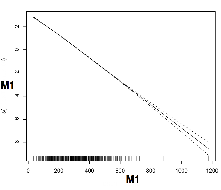
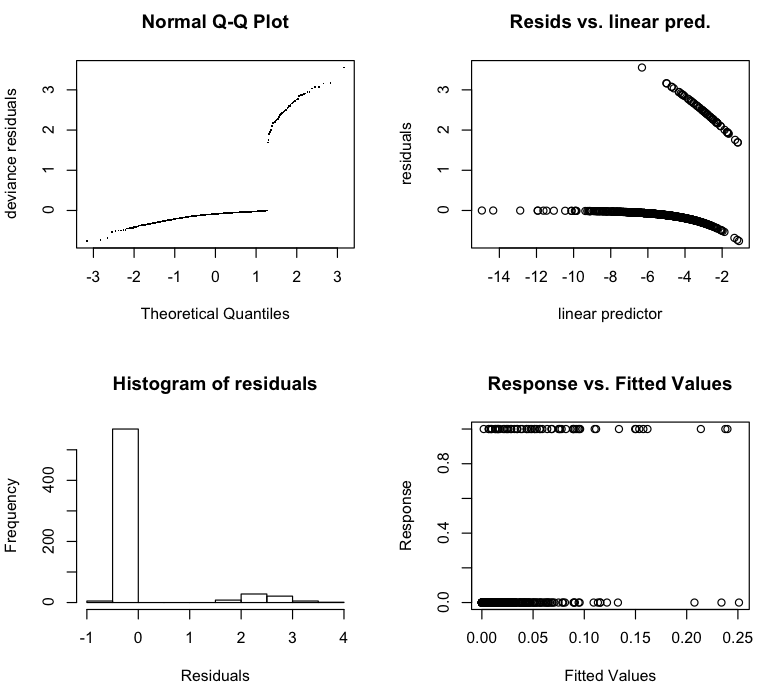
I suspect I may have messed up something fairly basic since M1 is the most obvious discriminator of the disease state. It is significant (as it should be) but the correlation is very low. Also, obviously, the model didn't converge (even when I increased iterations from 20->50). And finally the check plots look pretty outrageous
Question
Have I made a basic syntax error? Is there some malicious component in my model I'm over looking? Any help would be greatly appreciated.
Further work
I would like to add another metabolite (M2) to the model and 2 covariates (Birthweight and Race). When I add M2 to the model I get an non-convergence error:
> b = gamm(D.binary ~ Time  + s(M1) + s(M2) ,
      random = list(ParticipantID = ~ 1 + Time),  niterPQL=20, correlation = corLin(),
      data = NEC_data, family=binomial(link="logit"))

 Maximum number of PQL iterations:  20
iteration 1
iteration 2
Error in lme.formula(fixed = fixed, random = random, data = data, correlation = correlation,  :
  nlminb problem, convergence error code = 1
  message = false convergence (8)
Any advice about moving into the multidimensional space would also be appreciated.
Addition
I also tried this model with the discrete disease classification (control: 0,1 disease: 2,3) and poisson noise.
> b = gamm(NEC ~ DPP  + s(DSLNT_ug.mL)  ,
+      random = list(ParticipantID = ~ 1 + DPP),  niterPQL=20,
+      data = NEC_data, family=poisson)

 Maximum number of PQL iterations:  20
iteration 1
iteration 2
...
iteration 19
iteration 20
Error in solve.default(pdMatrix(a, factor = TRUE)) :
  system is computationally singular: reciprocal condition number = 3.13906e-19
