forecast using arima models [closed]

Question

I am trying to predict values using arima(0,1,1). After doing predict(mod,n.ahead=5) (in R) am getting the same value for all the predictions:

5947.681 5947.681 5947.681 5947.681 5947.681 

Is it correct?

Answer 1

In the future please provide a reproducible example for a question such as yours, as I don't have any idea on the characteristics of your data set. As @Irishstat mentions your data might not have a trend/pattern and could have a level shift.

Expanding my comment:

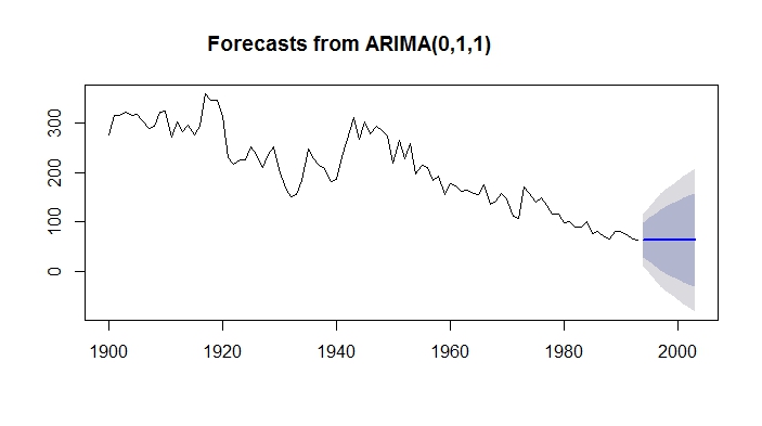
arima(0,1,1) is a simple exponential smoothing. The level of the forecast would be flat i.e., last value of the actual.

Below is an example illustrating my comment.

library("fma")
library("forecast")

## Without Drift
fit.m <- Arima(eggs,order = c(0,1,1))
forecast.m <- plot(forecast(fit.m,h=10))

#with Drift
fit.t <- Arima(eggs,order = c(0,1,1),include.drift=TRUE)
forecast.t <- plot(forecast(fit.t,h=10))

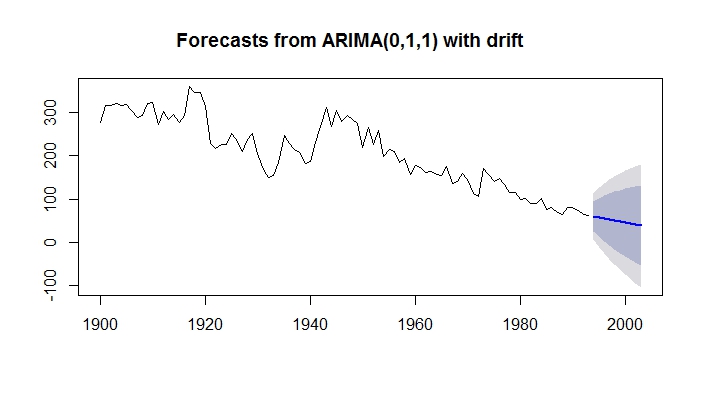
As you can see the first model without drift does not capture the downward trend. The forecast is flat.

forecast.m$mean
Time Series:
Start = 1994 
End = 2003 
Frequency = 1 
 [1] 62.87244 62.87244 62.87244 62.87244 62.87244 62.87244 62.87244 62.87244 62.87244 62.87244

The second model with drift term captures the downward trend as it includes drift term:

forecast.t$mean
Time Series:
Start = 1994 
End = 2003 
Frequency = 1 
 [1] 60.13606 57.75869 55.38132 53.00396 50.62659 48.24922 45.87186 43.49449 41.11712 38.73976

Answer 2

As you note, the forecasts for your $\text{ARIMA}(0,1,1)$ are constant. Nothing is amiss.

Let's begin by considering the differenced series. This is the simple case of an $\text{MA}(1)$ model with $0$ mean: $y(t) = \varepsilon(t) + θ\, \varepsilon(t-1)$.

If we're at time $T$, we have for the forecast of the observation at $T+1$:

$E[y_{T+1|T}] = E[\varepsilon_{T+1|T}] + θ E[\varepsilon_{T|T}] = 0 + θ \, \hat{\varepsilon}_{T|T}$

The last term, $\hat{\varepsilon}$, is a function of the data, but its exact form doesn't matter for our present purpose; it's just some forecasted value.

Now, let's forecast the next one:

$E[y_{T+2|T}] = E[\varepsilon_{T+2|T}] + θ E[\varepsilon_{T+1|T}] = 0 + θ\cdot 0 = 0$

... and similarly, all subsequent forecasts are $0$.

Now for an integrated $\text{MA}$, those are the predicted differences of the series. So for the undifferenced predictions, once you have the first forecast, all additional forecasts are equal to it.

Similarly, if you had, for example, an $\text{ARIMA}(0,1,2)$ model, then the second forecast would differ from the first and then all subsequent forecasts would be constant.

Answer 3

A characteristic of the model (simple exponential smoothing) that you are using is that forecasts are identical for every period in the future irrespective of the particular value of the ma(1) coefficient. This would also be true for a model that simply had a constant (mean model) or a recent level shift (last local mean)