Clarification on calculating odds ratios for interaction between continuous variables

Question

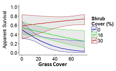
I know this or a similar question has been addressed more than once on CV, and I've tried to read/understand the responses, but I'm still stuck and hoping for some further clarification.

Results from a mark-recapture analysis that uses a logit link to model survival probability. This is the raw output from the model, so the estimates represent change on the logit(response) (i.e., I haven't back-transformed):

                 estimate     se        lcl        ucl
S:(Intercept)  -0.7805226 0.7506744 -2.2518445  0.6907993
S:grass        -4.6189001 2.0282830 -8.5943350 -0.6434653
S:shrub         0.0120384 0.0295291 -0.0458387  0.0699155
S:season2014    0.7729132 0.5820680 -0.3679401  1.9137665
S:grass:shrub   0.1835990 0.0894282  0.0083198  0.3588782

I want to get mean, LCL and UCL odds ratios for the interaction, grass*shrub. I understand there isn't one OR that represents the entire interaction, since the OR depends on the values of the covariates. I am primarily interested in holding shrub constant and calculating an OR +/- error for grass.

I attempted to follow this helpful post (How to interpret interaction continuos variables in logistic regression?) and my OR's for the mean make sense given my probability estimates (assuming that's a useful comparison to be making). However, when I apply the same steps to the LCL and UCL, the estimates are far from what I would expect.

For example
1) When shrub = 0, a unit change in grass is associated with a (exp(-4.62)-1)*100 = -99% decrease in odds of survival.

2) For every one unit increase in shrub, the effect of grass increases by (exp(0.18)-1)*100 = 19.72%.

(exp(.18)=1.19, exp(-4.62) = 0.0098)
3) The OR for grass when shrub = 1 is 1.19^1 * 0.0098 = 0.01.
- When shrub = 15: 1.19^15 * 0.0098 = 0.15
- When shrub = 30: 1.19^30 * 0.0098 = 2.18

However, when I apply these same steps to the LCL the OR is always essentially zero.
- When shrub = 1: 1.01^1 * 0.0002 = 0.0002
- When shrub = 15: 1.01^15 * 0.0002 = 0.0002
- When shrub = 30: 1.01^30 * 0.0002 = 0.0003

The OR's are huge when I calculate them for the UCL, e.g.:
When shrub = 30, OR = 25848.

I'm using these probability predictions (+/- 95% CI) from this model to help determine my expectation for the OR's, but maybe that's part of my problem. Based on this plot, I would expect the OR for grass to be at least marginally significantly positive (LCL of OR >=1) at the highest values of shrub cover, but that's far from what the OR's are showing above:

Am I calculating or interpreting the OR's incorrectly?
Does the method I'm using not apply to LCL and UCL? If so, what is the alternative/preferred method?
Am I just really bad at math?

Answer 1

To allow for much more general cases where the two interacting predictors can have multiple categories or be continuous and expanded into multiple terms (e.g., regression splines), I find the concept of requesting differences in predicted values and corresponding variance to be useful. The R rms package makes this way of thinking easy to execute. Suppose you had a logistic model with predictors x1 and x2 that are allowed to be nonlinear (using restricted cubic splines) and there is a general tensor spline interaction surface. Suppose we wanted to estimate the difference in the effect of x1 when varied from 10 to 20 for when x2=100 compared with x2=105. The following code would estimate this interaction effect (double difference).

require(rms)
f <- lrm(y ~ rcs(x1,4) * rcs(x2, 4))
contrast(f, list(x1=20, x2=100),   # a
            list(x1=10, x2=100),   # b
            list(x1=20, x2=105),   # c
            list(x1=10, x2=105))   # d

The contrast is (a - b) - (c - d). Confidence intervals and a test statistic are also printed, and there is an option to obtain simultaneous confidence intervals if many contrasts are suggested so that the resulting contrast is a vector instead of the single value exemplified here.

Answer 2

I posted this same question on the phidot forum (after a ~week of no replies here). Jeff Laake gave an excellent/thorough answer and noted that I need to incorporate the covariance of the betas in order to estimate the variance of the odds ratio.

Note that there is one error in his variance formula, which he points out later in the thread.
var(log(O) = ..... - 2s(cov(b1, B3)),
should be: var(log(O) = ..... + 2s(cov(b1, B3))

There's also some R code that is compatible with RMark.

http://www.phidot.org/forum/viewtopic.php?f=1&t=3051

Joe