How are the Control Limit Table constants calculated?

Question

For reference: https://controls.engin.umich.edu/wiki/images/3/39/Control_chart_constants.jpg

In a given set of manufacturing data, you can determine the control limits for 3-sigma confidence by the following equation: CL = Mean (X) +/- 3 * Standard deviation (population, sigma) / sqrt(# of samples). Now, if you don't have the population standard deviation, there's another way of calculating it: CL = X +/- (A2)*Range (R).

I'm trying to figure out how A2 (A constant from the given table) is calculated. What I have so far is a few things:

1) My google-fu has only demonstrated how to apply the process, not how the table is derived - too many results on "how to do it" makes it very difficult to actually find the derivation. Some mention that a derivation exists, but doesn't give the HOW.

2) X+/-3 *Sigma/(sqrt(n)) = X +/- (A2)*R 3*Sigma/(sqrt(n))=A2*R Given that A2 changes based off of N, but not at the rate of the sqrt(n), and that calculating a population standard deviation requires a lot more than we have, I've come up with a few guesses, and one sure-thing

Sure thing: This is an estimation, but a close enough one that it doesn't matter. Guess: There's a way to estimate population standard deviation based off of the range and the medium, that gets more and more accurate as we add more samples. Given that the standard deviation calculation requires more precise numbers.

I'm having trouble with the last step, putting it all together. I read the similar questions, but they don't quite get there. It'd also be nice to know with what confidence we have on the chart given.

Thank you

Answer 1

The math behind control limits like this can get quite deep without providing a lot of insight. You can confirm these limits for yourself with a simple Monte Carlo simulation. Generate a few random sets of data from a population with a known standard deviation, and compute the range. The range itself will exhibit a certain distribution. We want an unbiased range - that is, over the long run we would like our estimate of the standard deviation from this method to be neither larger nor smaller than the actual standard deviation.

Here is a simple Python program to demonstrate how you might go about this. You don't really need to understand Python to see what is going on here:

# compute standard deviation from sample range
# using simple Monte Carlo method

# the normal distribution we will use:
mu= 16.1
sigma = 3.45

# generate nx100 random samples from this population
# with different size n=2...15

# first we have to import some libraries we will use
import numpy as np

N = 10000
for n in range(2,16):
    # generate n x N samples:
    sample = np.random.normal(loc=mu, scale=sigma, size=(n,N))
    # find the range of each sample
    sampleMin = np.min(sample, 0) # take minimum of axis 0: once for each of N samples
    sampleMax = np.max(sample, 0) # ditto for the max
    sampleRange = sampleMax-sampleMin # the range - this is an array of N values
    rangeMean = np.mean(sampleRange) # the mean of these N values
    print 'n = %2d, scale factor %.3f'%\
      (n, 3*sigma/(rangeMean*np.sqrt(n))) # print the calculated factor 

This produces the following output:

n =  2, scale factor 1.893
n =  3, scale factor 1.021
n =  4, scale factor 0.733
n =  5, scale factor 0.578
n =  6, scale factor 0.485
n =  7, scale factor 0.419
n =  8, scale factor 0.372
n =  9, scale factor 0.337
n = 10, scale factor 0.308
n = 11, scale factor 0.287
n = 12, scale factor 0.267
n = 13, scale factor 0.249
n = 14, scale factor 0.235
n = 15, scale factor 0.224

As you can see, the numbers in the last column look an awful lot like the A2 values in your table. The difference will get smaller as you use a larger value for N - but it is practically insignificant.

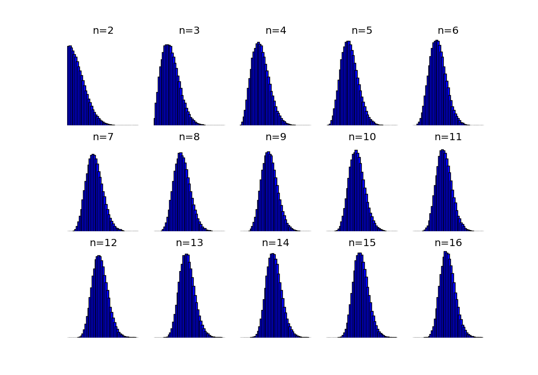
UPDATE here is a histogram showing how the distribution of the range changes with n. For n=2, the distribution is extremely asymmetric: as n gets bigger, the distribution becomes (unsurprisingly) more Gaussian.