3
$\begingroup$

I've been getting very odd factors in more complex models and simplify to this minimal case that behaves oddly vs my intuition.

Suppose we have the generative model, where everything is IID Normal

$A \sim N(0,1)$ $B \sim N(0,1)$

$Y_1 = A + \epsilon$ ; $Y_2 = A + \epsilon$ ; $Y_3 = A + \epsilon$

$X_1 = A + B + \epsilon$ ; $X_2 = A + B + \epsilon $ ; $X_3 = A + B + \epsilon$

Where each $\epsilon$ is independant, and in practice we divide by $Y$ and $X$ by $\sqrt{2}$ and $\sqrt{3}$ respectively to standardize.

The task is then to find the latent factors $A$ and $B$ from observed $X$s and $Y$s, pretending of course that we don't know the coefficients happen to all be 1.0, but we do know that $Y$ contains no $B$

This should be perfect for SEM/CFA, but when I try it fails to correctly identify factor A by an amount that can be corrected manually (so the solution does exist!). I'm using lavaan, and can't tell if it is a flaw in the software, the method, or my understanding.

In code:

library(lavaan)
library(data.table)

N = 100000

DT =  data.table(A = rnorm(N), B = rnorm(N))

DT[, Y1 := (A + rnorm(N))/sqrt(2)]
DT[, Y2 := (A + rnorm(N))/sqrt(2)]
DT[, Y3 := (A + rnorm(N))/sqrt(2)]
DT[, X1 := (A + B + rnorm(N))/sqrt(3)]
DT[, X2 := (A + B + rnorm(N))/sqrt(3)]
DT[, X3 := (A + B + rnorm(N))/sqrt(3)]

model = 'FA =~ Y1 + Y2 + Y3 + X1 + X2 + X3
FB =~ X1 + X2 + X3
FA ~~ 0*FB
'

fit = sem(model, data= DT, std.lv = TRUE, std.ov = FALSE)
summary(fit)

and the summary of our fit is

lavaan (0.5-20) converged normally after  20 iterations

  Number of observations                        100000

  Estimator                                         ML
  Minimum Function Test Statistic                9.770
  Degrees of freedom                                 6
  P-value (Chi-square)                           0.135

Parameter Estimates:

  Information                                 Expected
  Standard Errors                             Standard

Latent Variables:
                   Estimate  Std.Err  Z-value  P(>|z|)
  FA =~                                               
    Y1                0.711    0.003  227.070    0.000
    Y2                0.708    0.003  226.475    0.000
    Y3                0.709    0.003  226.770    0.000
    X1                0.580    0.003  176.083    0.000
    X2                0.577    0.003  175.597    0.000
    X3                0.579    0.003  176.073    0.000
  FB =~                                               
    X1                0.579    0.003  183.034    0.000
    X2                0.580    0.003  183.912    0.000
    X3                0.575    0.003  181.946    0.000

Covariances:
                   Estimate  Std.Err  Z-value  P(>|z|)
  FA ~~                                               
    FB                0.000                           

Variances:
                   Estimate  Std.Err  Z-value  P(>|z|)
    Y1                0.498    0.003  160.623    0.000
    Y2                0.497    0.003  161.192    0.000
    Y3                0.497    0.003  160.910    0.000
    X1                0.333    0.002  141.244    0.000
    X2                0.329    0.002  139.731    0.000
    X3                0.337    0.002  143.257    0.000
    FA                1.000                           
    FB                1.000                           

So far so good, but if we take the scores for those factors then they are not uncorrelated! Furthermore, if we regress Y1 on those factors, then Y1 appears to depend on factor B, which we specified is not the case.

DT = cbind(DT, predict(fit))

DT[, cor(FB, FA)]
#[1] 0.2219724

summary(DT[, lm(Y1 ~ FA + FB)])


Call:
lm(formula = Y1 ~ FA + FB)

Residuals:
     Min       1Q   Median       3Q      Max 
-2.67157 -0.39035  0.00245  0.38889  2.32116 

Coefficients:
             Estimate Std. Error t value Pr(>|t|)    
(Intercept) -0.002491   0.001823  -1.367    0.172    
FA           0.945142   0.002102 449.682   <2e-16 ***
FB          -0.231733   0.002351 -98.586   <2e-16 ***
---
Signif. codes:  0 ‘***’ 0.001 ‘**’ 0.01 ‘*’ 0.05 ‘.’ 0.1 ‘ ’ 1

Residual standard error: 0.5764 on 99997 degrees of freedom
Multiple R-squared:  0.6691,    Adjusted R-squared:  0.6691 
F-statistic: 1.011e+05 on 2 and 99997 DF,  p-value: < 2.2e-16

There does appear to be a correct solution though, because if we take those regression coefficients and make a new factor A, then orthogonality is achieved and the Ys all only depend on this new factor

DT[, CA := 0.94*FA - 0.235*FB]

DT[, cor(CA,FB)]
#[1] -0.00160991

What is going on?

EDIT

As far as I can tell, it is fitting the weights correctly, this diagram purports to show the fitted model (semPaths) and the residual variances and loadings all look correct. So perhaps it is the predict function where the issue lies?

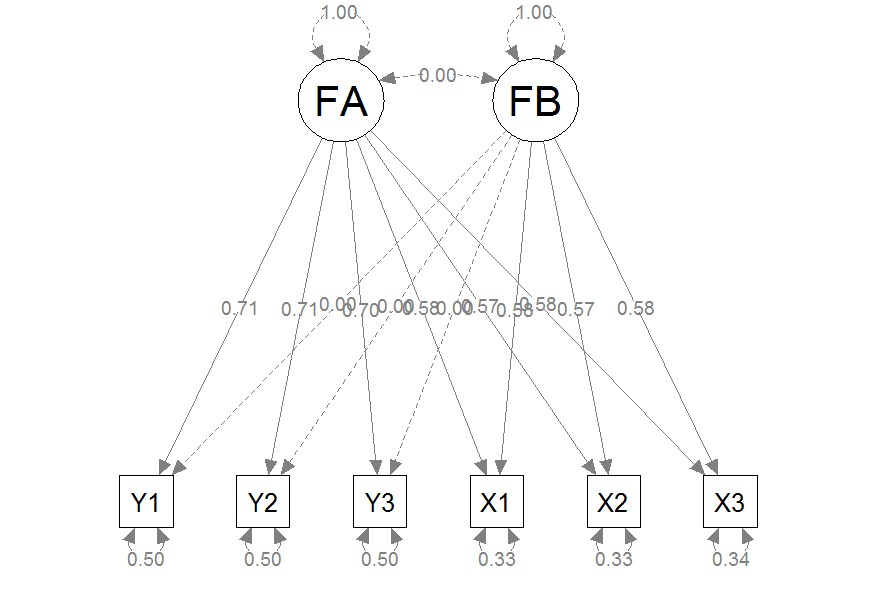
SEMdiagram

$\endgroup$
4
  • $\begingroup$ Can you draw the path diagram you are trying to fit? $\endgroup$
    – AdamO
    Commented Jan 26, 2016 at 1:10
  • $\begingroup$ Why is $F_b \perp F_a$? $\endgroup$
    – AdamO
    Commented Jan 26, 2016 at 1:10
  • $\begingroup$ We know $F_A$ and $F_B$ are orthogonal from the problem definition - A and B are independent N(0,1). In the real world case, we simply have reason to believe these are completely unconnected factors. $\endgroup$
    – Corvus
    Commented Jan 26, 2016 at 8:07
  • $\begingroup$ @AdamO I could draw the path diagram I'm attempting to fit, or that lavaan is fitting, but ultimately the more important question would be what is the correct path diagram for the generative model described. $\endgroup$
    – Corvus
    Commented Jan 26, 2016 at 8:08

2 Answers 2

1
$\begingroup$

You see a relationship between $Y_1$ and the latent factors $F_a$ and $F_b$ because of the indirect effect of having $F_a$ and $F_b$ manifested by $X$s which are manifested by $A$. If you drew the diagram, you'd see you don't have a proper DAG. If you want orthogonal components, why not set the loadings of $X$ to 0 in the manifestation of $F_a$?

$\endgroup$
1
  • $\begingroup$ I've tried that, omitting them from the formula is the same as setting the loading to zero in this case. The fit is identical. Likewise, I am specifying that FA and FB are orthogonal, but they are not coming out as that in the fit? $\endgroup$
    – Corvus
    Commented Jan 26, 2016 at 7:52
1
$\begingroup$

It appears my problem here is with a basic misunderstanding between factor scores and factor score estimates.

Factors A and B are indeed uncorrelated, but these are the latent hidden factors which are never computed in the model fit. The fitted model shows all the correct weightings between the latent variables and observables. The problem only appears when looking at the result of predict.

Predict tries to estimate the factor scores from the data, using a procedure like this described here: Mplus documentation

This paper discusses estimating scores for the related method of EFA, and discusses the pros and cons of different methods. In particular noting that although the factors are uncorrelated, it may well be that the estimates of those factors are in fact correlated (e.g. Bartlett Scores and Regression Scores).

There are, it seems, methods to estimate the factors which force the estimates to have the same correlation properties as the true factors, but this reduces the accuracy with which they estimate the true latent factor.

Basically there appears to be an analogy between bias-variance trade off, of bias-covariance trade off. You can either estimate the individual factors more accurately, but get the covariances wrong, or get the covariances right and the factor scores more wrong.

$\endgroup$

Your Answer

By clicking “Post Your Answer”, you agree to our terms of service and acknowledge you have read our privacy policy.

Not the answer you're looking for? Browse other questions tagged or ask your own question.