Categorical solution
Treating the values as categorical loses the crucial information about relative sizes. A standard method to overcome this is ordered logistic regression. In effect, this method "knows" that $A\lt B\lt \cdots \lt J\lt \ldots$ and, using observed relationships with regressors (such as size) fits (somewhat arbitrary) values to each category that respect the ordering.
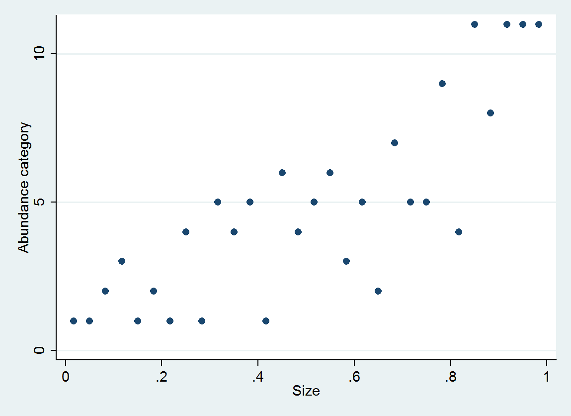
As an illustration, consider 30 (size, abundance category) pairs generated as
size = (1/2, 3/2, 5/2, ..., 59/2)
e ~ normal(0, 1/6)
abundance = 1 + int(10^(4*size + e))
with abundance categorized into intervals [0,10], [11,25], ..., [10001,25000].

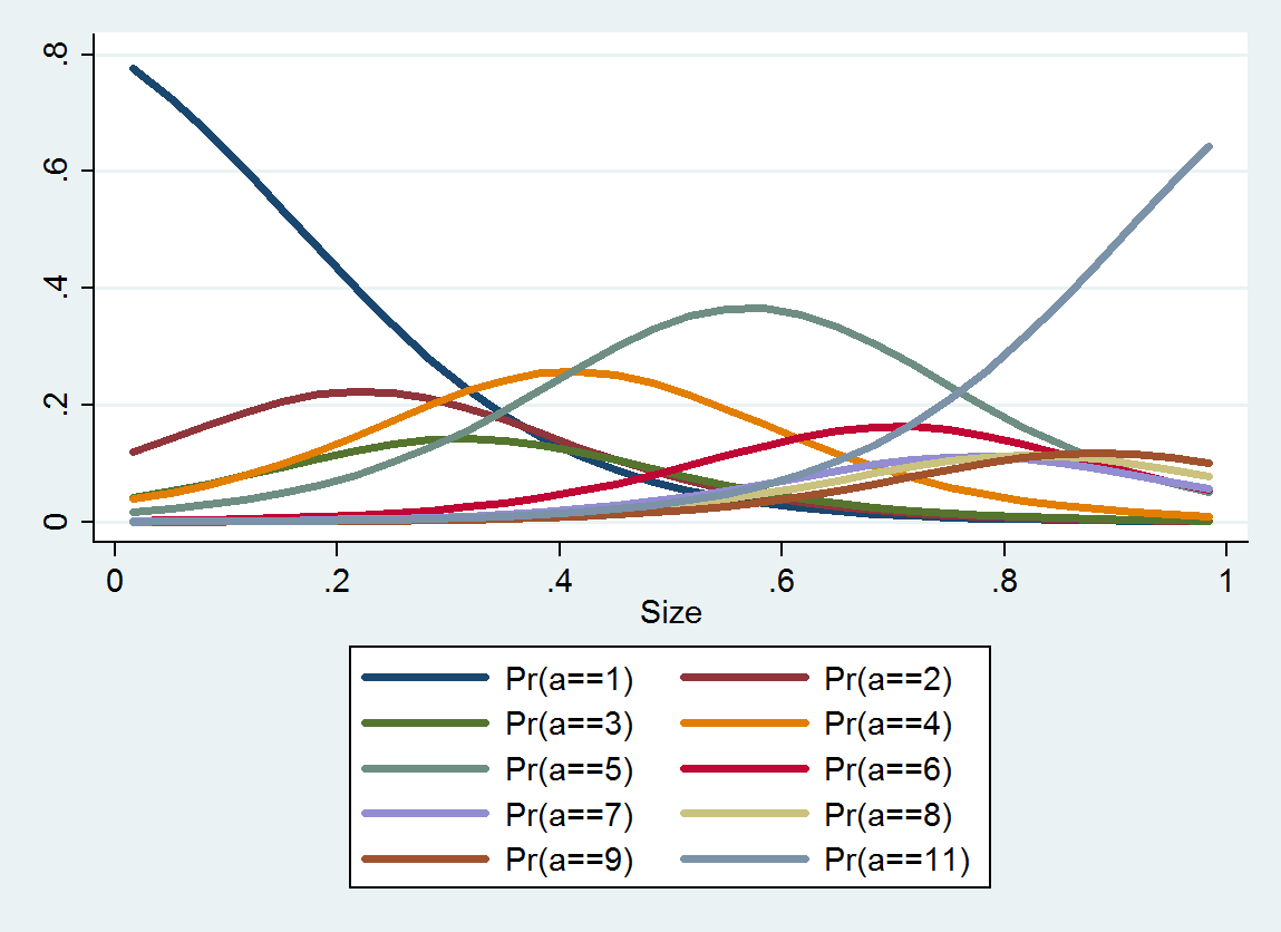
Ordered logistic regression produces a probability distribution for each category; the distribution depends on size. From such detailed information you can produce estimated values and intervals around them. Here is a plot of the 10 PDFs estimated from these data (an estimate for category 10 was not possible due to lack of data there):

Continuous solution
Why not select a numeric value to represent each category and view the uncertainty about the true abundance within the category as part of the error term?
We can analyze this as a discrete approximation to an idealized re-expression $f$ which converts abundance values $a$ into other values $f(a)$ for which the observational errors are, to a good approximation, symmetrically distributed and of roughly the same expected size regardless of $a$ (a variance-stabilizing transformation).
To simplify the analysis, suppose the categories have been chosen (based on theory or experience) to achieve such a transformation. We may assume then that $f$ re-expresses the category cutpoints $\alpha_i$ as their indexes $i$. The proposal amounts to selecting some "characteristic" value $\beta_i$ within each category $i$ and using $f(\beta_i)$ as the numerical value of abundance whenever the abundance is observed to lie between $\alpha_i$ and $\alpha_{i+1}$. This would be a proxy for the correctly re-expressed value $f(a)$.
Suppose, then, that abundance is observed with error $\varepsilon$, so that the hypothetical datum is actually $a+\varepsilon$ instead of $a$. The error made in coding this as $f(\beta_i)$ is, by definition, the difference $f(\beta_i) - f(a)$, which we can express as a difference of two terms
$$\text{error} = f(a + \varepsilon) - f(a) - \left(f(a + \varepsilon) - f(\beta_i)\right).$$
That first term, $f(a + \varepsilon) - f(a)$, is controlled by $f$ (we can't do anything about $\varepsilon$) and would appear if we did not categorize aboundances. The second term is random--it depends on $\varepsilon$--and evidently is correlated with $\varepsilon$. But we can say something about it: it must lie between $i - f(\beta_i) \lt 0$ and $i+1 - f(\beta_i) \ge 0$. Moreover, if $f$ is doing a good job, the second term might be approximately uniformly distributed. Both considerations suggest choosing $\beta_i$ so that $f(\beta_i)$ lies halfway between $i$ and $i+1$; that is, $\beta_i \approx f^{-1}(i+1/2)$.
These categories in this question form an approximately geometric progression, indicating that $f$ is a slightly distorted version of a logarithm. Therefore, we should consider using the geometric means of the interval endpoints to represent the abundance data.
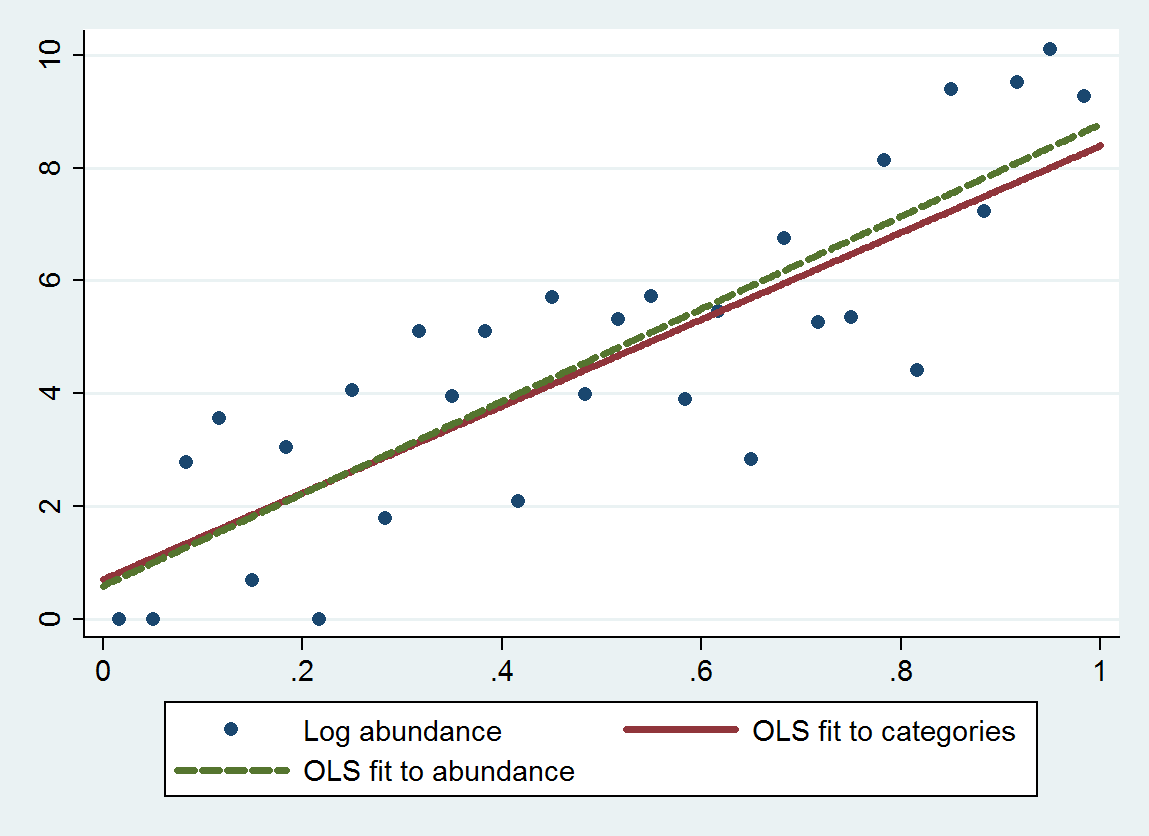
Ordinary least squares regression (OLS) with this procedure gives a slope of 7.70 (standard error is 1.00) and intercept of 0.70 (standard error is 0.58), instead of a slope of 8.19 (se of 0.97) and intercept of 0.69 (se of 0.56) when regressing log abundances against size. Both exhibit regression to the mean, because theoretical slope should be close to $4 \log(10) \approx 9.21$. The categorical method exhibits a bit more regression to the mean (a smaller slope) due to the added discretization error, as expected.

This plot shows the uncategorized abundances along with a fit based on the categorized abundances (using geometric means of the category endpoints as recommended) and a fit based on the abundances themselves. The fits are remarkably close, indicating this method of replacing categories by suitably chosen numerical values works well in the example.
Some care usually is needed in choosing an appropriate "midpoint" $\beta_i$ for the two extreme categories, because often $f$ is not bounded there. (For this example I crudely took the left endpoint of the first category to be $1$ rather than $0$ and the right endpoint of the last category to be $25000$.) One solution is to solve the problem first using data not in either of the extreme categories, then use the fit to estimate appropriate values for those extreme categories, then go back and fit all the data. The p-values will be slightly too good, but overall the fit should be more accurate and less biased.

