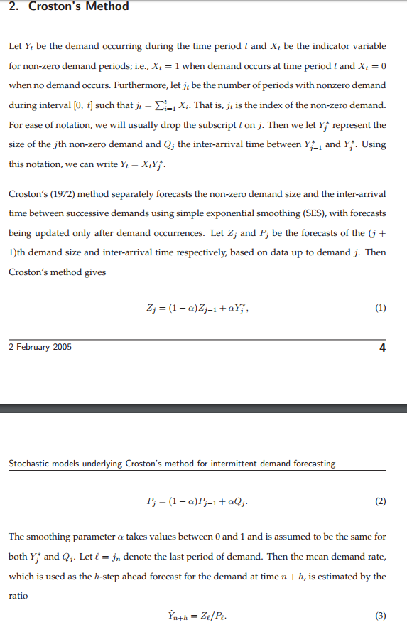
OK, let's use your data: $y_1=0, y_2=1, y_3=\dots=y_{10}=0$.
The problem is that Croston's method only updates its state variables whenever there is a nonzero demand. In our case:
- The inter-arrival time state is initialized as $P_1=2$, because the first nonzero demand occurred in the second time period. After that, it is not updated, because there is no other nonzero demand.
- The demand size state is initialized as $Q_1=1$, because the first nonzero demand was of size 1. After that, it is not updated, because there is no other nonzero demand.
The point forecast right after this initialization in period 2 would therefore be $Q_1/P_1=0.5$. And since nothing is updated as long as there is no new nonzero demand, the point forecast stays at this value until a new demand occurs.
Now, one might of course object that this makes no sense and that (say) we would want the inter-arrival time state to be updated more often, say after every time period. However, this runs into the problem that your forecast will be too high right after a nonzero demand, and too low after many nonzero demands. This is essentially the same problem as you see if you apply Single Exponential Smoothing to intermittent demands.
In our example, we only observed ten data points. Croston's method is designed to catch changes in the dynamics of the intermittent time series we are looking at. Question: will we even be able to detect changing dynamics in a time series that is (a) very short and (b) carries very little signal? I'd say no.
So my recommendation would be: think about the length of the time series you have, and about the specific things whose demand you are forecasting. If your series are so short that you likely won't be able to detect changes in dynamics, don't use Croston's method. Instead, use a simple arithmetical average of past sales, which would in this case give you a forecast of $1/10$.
Here are a few earlier thoughts of mine on intermittent and count data forecasting.

