3
$\begingroup$

I was thinking a bit about confusion matrices and it came to my mind the determinant of a confusion matrix could be an useful performance metric in classification.

Indeed, I got some results in Google about it, such as this book and this study using it.

The basic idea is the ratio of the determinant of the confusion matrix and the determinant of the perfect solution is $\in\{-1,1\}$.

Is it useful though? I mean, it's possible to achieve the ratio equal to $1$ with a perfect match between classes in solution and response, but the labels themselves don't have to match, like this example:

sol = iris$Species
res = iris$Species[c(101:150, 1:100)]
res.tab = table(sol, res)
res.tab

#            res
#sol          setosa versicolor virginica
#  setosa          0          0        50
#  versicolor     50          0         0
#  virginica       0         50         0

sol.tab = table(sol,sol)
det.res = det(as.matrix(as.data.frame.matrix(res.tab)))
det.sol = det(as.matrix(as.data.frame.matrix(sol.tab)))
det.res/det.sol

#> det.res/det.sol
#[1] 1

Accuracy is exactly $0$ in this case, yet the determinant ratio is $1$. Of course, switching labels around would get us 100% accuracy, but I'm sure that's not good practice (unless your model learns when to do it, but them the resulting confusion matrix would not be the same).

$\endgroup$
2
  • 3
    $\begingroup$ This is a strange question. You suggest a procedure without supplying any basis for it, offer an example showing how awful it can be, and then ask "is it useful?" What kind of answers do you expect? $\endgroup$
    – whuber
    Commented Jul 15, 2016 at 18:03
  • 1
    $\begingroup$ @whuber The "basis" is it's actually being used. The example is analogous to accuracy (you can find questions about the flipping procedure here on stats). I expect answers about if it can be useful in multiclass classification, imbalanced classes, or any other application out of the idealized binary, equal sized, classes. $\endgroup$
    – Firebug
    Commented Jul 15, 2016 at 18:15

3 Answers 3

2
$\begingroup$

The determinant of a confusion matrix probably isn't useful as an accuracy metric.

Determinants are usually used when the matrix is an operator, and confusion matrices aren't operators. Yes, they are matrices, but that's just because matrices provide a convenient way to organizing the classification information.

$\endgroup$
1
  • 1
    $\begingroup$ the MCC measure (an alternative to F1) has the determinant as its numerator: safjan.com/difference-between-matthews-and-f1 You can think of the confusion matrix as mapping a distribution of true positives and negatives (p, q) to a distribution of observations. $\endgroup$
    – Att Righ
    Commented Aug 18, 2023 at 14:13
2
$\begingroup$

Only found this question now as a colleague asked it and I tried to find an answer. So I'll share what I told him after some consideration. It is a rather geometric explanation.

The confusion matrix has two degrees of freedom, as the total number of negative classes (TN + FP) and the total number of positive classes (FN + TP) is fixed.

TN FP
FN TP

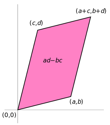
determinant in geometry

The determinant is measuring the (oriented) area of a parallelogram. Thinking about this geometry you can draw the prediction vectors (a=TN,b=FN) and (c=FP,d=TP) of the confusion matrix, which makes the x1-axis the negative classes and the x2-axis the positive classes. As their total numbers are fixed, the long diagonal of the parallelogram is fixed, and if you base it at (0,0) the top right vertex is fixed (a+c=TN+FP=total negative classes, b+d=FN+TP=total positive classes). The ideal solution is a rectangle. And we note that no parallelogram can have a larger area than a rectangle (as the diagonal is fixed and our vectors all consist of positive integers). So far so good, the ideal solution has the largest value in our metric.

This geometric picture also allows to reason about data skew. A skewed dataset will have a very slim rectangle as the ideal solution. If you get one of the less frequent class wrong, this moves the corner of our parallelogram one step along the short edge, thus reducing a large chunk of area. Whereas getting the frequent class wrong moves the point along the long edge, thus only slightly reducing the area.

And as you noted the determinant does generalize nicely to higher dimensions, i.e. multiclass classification. It now measures the (oriented) volume of a paralleletope. Again the same considerations about skewness hold.

Now, as you also noted, the only property of the determinant that is somewhat unneeded is that it is alternating. So shuffling two labels just multiplies it by -1. I'd argue that this does not play a role in practice due to two reasons:

  • if you see a classifier like in your example you would just shuffle the labels and have a perfect classifier
  • if you have a skewed dataset you will not even be able to create such an example

So the main geometric insight is that applying a determinant to a (multi-class) classification problem can be translated to how much of an orthotope is covered by a paralleletope.

$\endgroup$
2
$\begingroup$

The determinant of the confusion matrix is proportional to the Matthews Correlation Coefficient (MCC, also called the phi coefficient). https://en.m.wikipedia.org/wiki/Phi_coefficient

So basically, the determinant of the confusion matrix is an unscaled measure of correlation. It’s not expected to be as useful as MCC because it doesn’t account for the total population size.

$\endgroup$

Your Answer

By clicking “Post Your Answer”, you agree to our terms of service and acknowledge you have read our privacy policy.

Not the answer you're looking for? Browse other questions tagged or ask your own question.