15
$\begingroup$

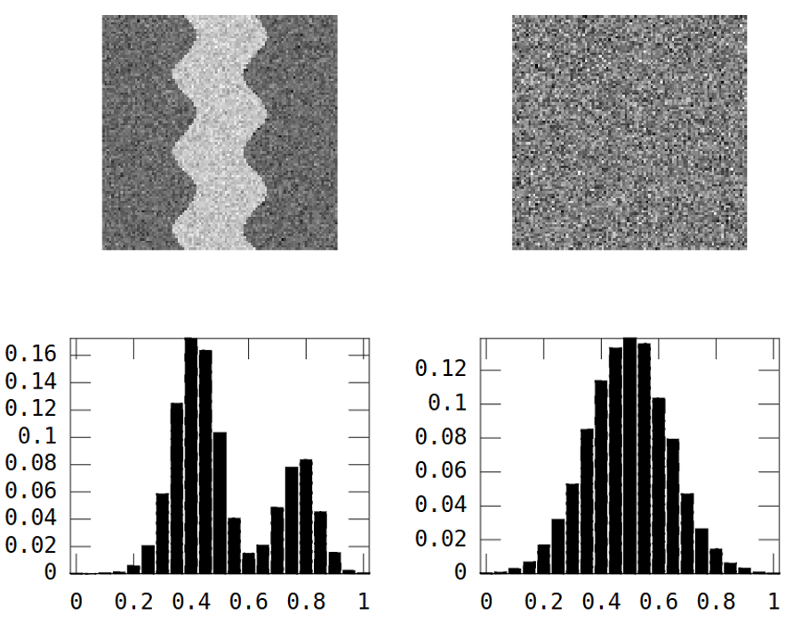
Consider these two grayscale images:
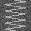
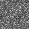
river random

The first image shows a meandering river pattern. The second image shows random noise.

I am looking for a statistical measure that I can use to determine if it is likely that an image shows a river pattern.

The river image has two areas: river = high value and everywhere else = low value.

The result is that the histogram is bimodal:
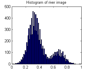
enter image description here

Therefore an image with a river pattern should have a high variance.

However so does the random image above:

River_var = 0.0269, Random_var = 0.0310

On the other hand the random image has low spatial continuity, whereas the river image has high spatial continuity, which is clearly shown in the experimental variogram: enter image description here
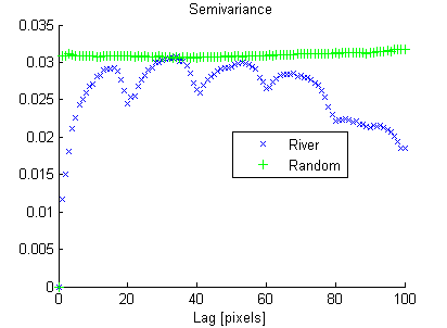
In the same way that the variance "summarizes" the histogram in one number, I am looking for a measure of spatial contiuity that "summarizes" the experimental variogram.

I want this measure to "punish" high semivariance at small lags harder than at large lags, so I have come up with:

$\ svar = \sum_{h=1}^n \gamma(h)/h^2 $

If I only add up from lag = 1 to 15 I get:

River_svar = 0.0228, Random_svar = 0.0488

I think that a river image should have high variance, but low spatial variance so I introduce a variance ratio:

$\ ratio = var/svar $

The result is:

River_ratio = 1.1816, Random_ratio = 0.6337

My idea is to use this ratio as a decision criteria for if an image is a river image or not; high ratio (e.g. > 1) = river.

Any ideas on how I can improve things?

Thanks in advance for any answers!

EDIT: Following the advice of whuber and Gschneider here are the Morans I of the two images calculated with a 15x15 inverse distance weight matrix using Felix Hebeler's Matlab function:
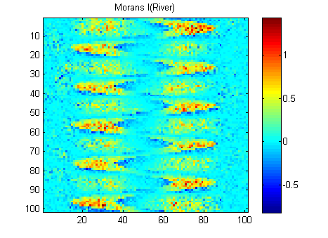
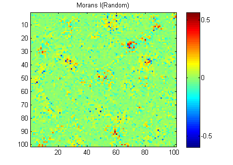
River_M Random_M

I need to summarize the results into one number for each image. According to wikipedia: "Values range from −1 (indicating perfect dispersion) to +1 (perfect correlation). A zero value indicates a random spatial pattern." If I sum up the square of the Morans I for all pixels I get:

River_sumSqM = 654.9283, Random_sumSqM = 50.0785 

There is a huge difference here so Morans I seem to be a very good measure of spatial continuity :-).

And here is a histogram of this value for 20 000 permutations of the river image: histogram of permuations
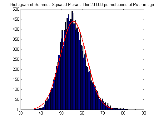
Clearly the River_sumSqM value (654.9283) is unlikely and the River image is therefore not spatially random.

$\endgroup$
6
  • 4
    $\begingroup$ Interesting question. One bit of advice that comes to mind immediately is to focus on the short-range part of the variogram: that is the crucial part and will do the best job distinguishing pairs of images like these. (Closely related statistics are Moran's I and Geary's C.) It's hard to give specific advice, though, unless you can more clearly characterize the kinds of images you anticipate processing. $\endgroup$
    – whuber
    Commented Jun 8, 2012 at 12:59
  • 2
    $\begingroup$ +1 whuber, Moran's I seems like a good start in this case. Then maybe consider a permutation test to see how "extreme" your image is. $\endgroup$
    – Gschneider
    Commented Jun 8, 2012 at 13:15
  • $\begingroup$ @Gschneider The permutation test is a nice idea, especially because no permutations need to be conducted! It's straightforward to calculate the distribution of the variogram (or Moran's I or Geary's C or whatever) under permutations of the values in the image: there are so many values that the CLT applies. (E.g., the variogram will look like the green points; twice their constant height is the variance of the image values.) The problem becomes more challenging when a "river" pattern needs to be distinguished from other patterns such as a "lake" or "rivers" can have widely varying widths. $\endgroup$
    – whuber
    Commented Jun 8, 2012 at 13:40
  • $\begingroup$ Sorry but I am not sure I follow: are you telling me to permute the image being tested pixel per pixel in some random fashion and then compare the Moran's I value of the permuted image with that of the image being tested? $\endgroup$
    – Andy
    Commented Jun 8, 2012 at 13:52
  • $\begingroup$ What I had in mind was first define some sort of (probably simple) neighborhood structure and compute Moran's I. Then you can compute K, say 200,000, possible permutations of the pixels, computing Moran's I for each permutation. Once you've got these 200,000 Moran's I, see where your observed statistic lies. But, whuber's method sounds easier :). $\endgroup$
    – Gschneider
    Commented Jun 8, 2012 at 16:27

3 Answers 3

3
$\begingroup$

I was thinking that a Gaussian blur acts as a low-pass filter leaving the large-scale structure behind and removing the high wave-number components.

You could also look at the scale of wavelets required to generate the image. If all the information is living in the small scale wavelets then it is likely not the river.

You might consider some sort of auto-correlation of one line of the river with itself. So if you took a row of pixels of the river, even with noise, and found the cross-correlation function with the next row, then you could both find the location and value of the peak. This value is going to be much higher than what you are going to get with the random noise. A column of pixels is not going to produce much of a signal unless you pick something from the region where the river is.

http://en.wikipedia.org/wiki/Gaussian_blur

http://en.wikipedia.org/wiki/Cross-correlation

$\endgroup$
4
  • 2
    $\begingroup$ Some interesting ideas here! Could I persuade you to flesh out this answer by applying one or more of your approaches to the sample images to (1) show how your methods work and (2) evaluate how well they perform? $\endgroup$
    – whuber
    Commented Mar 26, 2013 at 15:43
  • 1
    $\begingroup$ It is from my Thesis. (Mechanical Engineering) I put a Gaussian blur on the position of a nonlinear pendulum, and then used the convolution method to back out the position from an image and compare it to the analytic. I tried it with several levels of noise. As long as the noise was below a threshold related to the size of the gaussian, there was very good reconstruction. link Figure 11 was the relevant graph for the reconstruction. Figure 6 and equation 2 indicate response to noise. $\endgroup$ Commented Mar 27, 2013 at 4:48
  • 1
    $\begingroup$ Thanks! So it looks like you are in a great position to flesh out this answer and demonstrate how effective it really is. :-) $\endgroup$
    – whuber
    Commented Mar 27, 2013 at 4:52
  • $\begingroup$ Sorry for the double comment. I think it is "clever" to use part of an object as a pseudo "mother-wavelet" for itself. It seems self referential, but also poetic. Self Adjoint. $\endgroup$ Commented Mar 27, 2013 at 4:54
3
$\begingroup$

This is a bit late, but I cannot resist one suggestion and one observation.

First, I believe a more "image processing" approach may be better suited than histogram/variogram analysis. I would say that the "smoothing" suggestion of EngrStudent is on the right track, but the "blur" part is counter-productive. What is called for is an edge-preserving smoother, such as a Bilateral filter, or a median filter. These are more sophisticated than moving average filters, as they are by necessity nonlinear.

Here is a demonstration of what I mean. Below are two images approximating your two scenarios, along with their histograms. (The images are each 100 by 100, with normalized intensities).

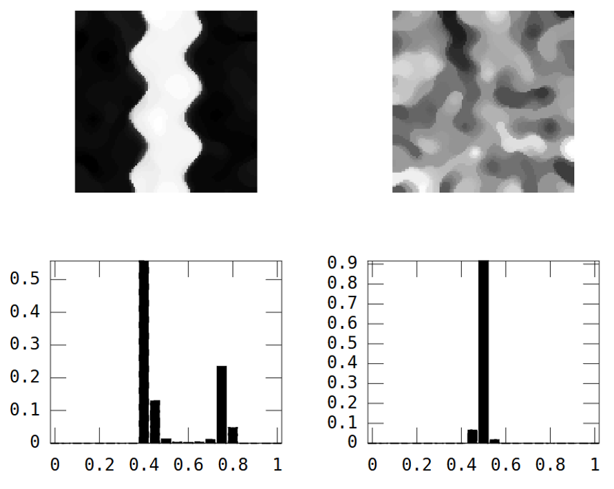
Raw Images raw images

For each of these images I then apply a 5 by 5 median filter 15 times*, which smooths the patterns while preserving the edges. The results are shown below.

Smoothed Images smoothed images

(*Using a larger filter would still maintain the sharp contrast across the edges, but would smooth their position.)

Note how the "river" image still has a bimodal histogram, but it is now nicely separated into 2 components*. Meanwhile, the "white noise" image still has a single-component unimodal histogram. (*Easily thresholded via, e.g. Otsu's method, to make a mask and finalize the segmentation.)


Second, your image is certainly not a "river"! Aside from the fact that it is too anisotropic (stretched in the "x" direction), to the extent that meandering rivers can be described by a simple equation, their geometry is actually much closer to a sine-generated curve than to a sine curve (e.g. see here or here). For low amplitudes this is approximately a sine curve, but for higher amplitudes the loops become "overturned" ($x\neq f[y]$), which in nature eventually leads to cutoff.

(Sorry for the rant ... my training was as a geomorphologist, originally)

$\endgroup$
1
  • $\begingroup$ On a side note, it is generally a good idea to be very cautious in applying "variogram methods" to natural images, which are typically not stationary. This is touched on in my answer here. $\endgroup$
    – GeoMatt22
    Commented Oct 14, 2016 at 3:34
0
$\begingroup$

A suggestion which may be a quick win (or may not work at all, but can easily be eliminated) - have you tried looking at the ratio of mean to variance of the image intensity histograms?

Take the random noise image. Assuming it's generated by randomly emitted photons (or similar) hitting a camera, and each pixel is equally likely to be hit, and that you have the raw readings (i.e. values are not rescaled, or are rescaled in a known way you can undo), then the number of readings in each pixel ought to be poisson distributed; you're counting the number of events (photons hitting a pixel) that occur in a fixed time period (exposure time) multiple times (over all pixels).

In the case where there's a river of two different intensity values, you have a mixture of two poisson distributions.

A really quick way to test an image then might be to look at the ratio of mean to variance of the intensities. For a poisson distribution the mean will approximately equal the variance. For a mixture of two poisson distributions, the variance will be bigger than the mean. You'll end up needing to test the ratio of the two against some pre-set threshold.

It's very crude. But if it works, you'll be able to calculate the necessary sufficient statistics with just one pass over each pixel in your image :)

$\endgroup$

Your Answer

By clicking “Post Your Answer”, you agree to our terms of service and acknowledge you have read our privacy policy.

Not the answer you're looking for? Browse other questions tagged or ask your own question.