Why is the James-Stein estimator called a "shrinkage" estimator?

Question

I have been reading about the James-Stein estimator. It is defined, in this notes, as

$$ \hat{\theta}=\left(1 - \frac{p-2}{\|X\|^2}\right)X$$

I have read the proof but I don't understand the following statement:

Geometrically, the James–Stein estimator shrinks each component of $X$ towards the origin...

What does "shrinks each component of $X$ towards the origin" mean exactly? I was thinking of something like $$\|\hat{\theta} - 0\|^2 < \|X - 0\|^2,$$ which is true in this case as long as $(p+2) < \|X\|^2$, since $$\|\hat{\theta}\| = \frac{\|X\|^2 - (p+2)}{\|X\|^2} \|X\|.$$

Is this what people mean when they say "shrink towards zero" because in the $L^2$ norm sense, the JS estimator is closer to zero than $X$?

Update as of 22/09/2017: Today I realized that perhaps I am over-complicating things. It seems like people really mean that once you multiply $X$ by something that is smaller than $1$, namely, the term $\frac{\|X\|^2 - (p + 2)}{\|X\|^2}$, each component of $X$ will be smaller than it used to be.

Answer 1

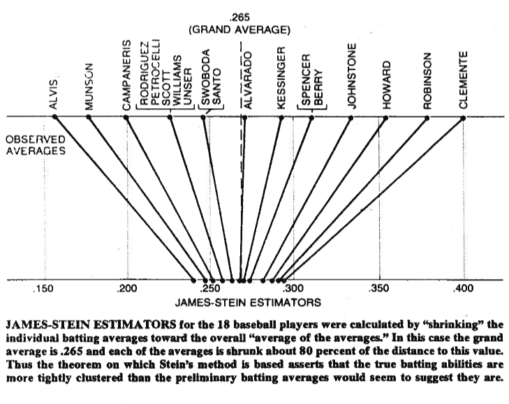
A picture is sometimes worth a thousand words, so let me share one with you. Below you can see an illustration that comes from Bradley Efron's (1977) paper Stein's paradox in statistics. As you can see, what Stein's estimator does is move each of the values closer to the grand average. It makes values greater than the grand average smaller, and values smaller than the grand average, greater. By shrinkage we mean moving the values towards the average, or towards zero in some cases - like regularized regression - that shrinks the parameters towards zero.

Of course, it is not only about shrinking itself, but what Stein (1956) and James and Stein (1961) have proved, is that Stein's estimator dominates the maximum likelihood estimator in terms of total squared error,

$$ E_\mu(\| \boldsymbol{\hat\mu}^{JS} - \boldsymbol{\mu} \|^2) < E_\mu(\| \boldsymbol{\hat\mu}^{MLE} - \boldsymbol{\mu} \|^2) $$

where $\boldsymbol{\mu} = (\mu_1,\mu_2,\dots,\mu_p)'$, $\hat\mu^{JS}_i$ is the Stein's estimator and $\hat\mu^{MLE}_i = x_i$, where both estimators are estimated on the $x_1,x_2,\dots,x_p$ sample. The proofs are given in the original papers and the appendix of the paper you refer to. In plain English, what they have shown is that if you simultaneously make $p > 2$ guesses, then in terms of total squared error, you'd do better by shrinking them, as compared to sticking to your initial guesses.

Finally, Stein's estimator is certainly not the only estimator that gives the shrinkage effect. For other examples, you can check this blog entry, or the referred Bayesian data analysis book by Gelman et al. You can also check the threads about regularized regression, e.g. What problem do shrinkage methods solve?, or When to use regularization methods for regression?, for other practical applications of this effect.