How to assess accuracy of phone GPS in measuring distances?

Question

I am a complete stranger to statistics (apart from mandatory courses in college), but lately I ran into an interesting real-world scenario.

Recently I started jogging. I take my GPS phone with me to measure time and distance. I picked a route (about 4km, but I don't know exactly) and started running. I have observed that the distance measured is not constant, although the route is the same. Sometimes, the distance measured is a little more than 4km and sometimes a little less. I am interested in the precision of my phone GPS.

But there is one small problem: when I arrive, I usually (but not always) check the phone, and if the distance is less than 4Km, I continue running to reach 4Km. So even though I have all the measurements saved in the history, I cannot use them to calculate the mean value, because sometimes I run a little bit more to reach 4km. What I do know, however, is that during my 20 runs, the minimum distance was about 3.9km and maximum 4.05km.

So what I am interested in is how precise my GPS is and how long the path is. I expect the answer to be something along the lines "with confidence X%, the path is Y km long and the GPS has Z% distance variation". Or would I have to know the exact mean to calculate that?

Answer 1

As I mentioned even though you cannot compute a confidence interval for the mean of the distribution you can determine a nonparametric tolerance interval. Tolerance interval tell you with a given level of confidence what percentage of the distribution of your run lengths fall within the interval. They are based on using upper and lower order statistics for the end point. Since you can say that the minimum distance out of 20 was 3.9 km and the maximum was 4.05 that range can be used as a tolerance interval for a certain confidence and coverage. Table A.16 in Hahn and Meeker's book "Statistical Intervals" provides the answer. From this we see that you can be 99% confident that the interval generated by taking the range will include at least 75% of the distribution. For it to be able to claim higher coverage you would need a larger sample size. For a sample size of 50 it will give you 99% confidence in a coverage of 90% of the distribution and for 95% you need a sample size of 100. For 99% confidence in 99% coverage you need a sample size of 500. The required sample size can go down a little for a given % coverage if you lower the ocnfidence level from 99% to say 95% or 90%.

Answer 2

The purpose of this answer is to elaborate on some special issues concerning GPS measurement, because they may present pitfalls for the unwary.

GPS readings vary over time: if you stay in one place, a phone reading (which is among the least accurate of GPS receivers) may change by several tens of meters (or more), depending on satellite availability, echoes from landscape clutter, and so on.

GPS accuracy varies with location, for many of the same reasons.

These two sources of variation tend to increase measured trip distances.

Estimates of lengths of trips tend to have a low bias for geometric reasons: the GPS records points periodically, thereby approximating a curvilinear route as a complicated "polyline." The polyline tends to cut corners, leading to an underestimate of total trip length.

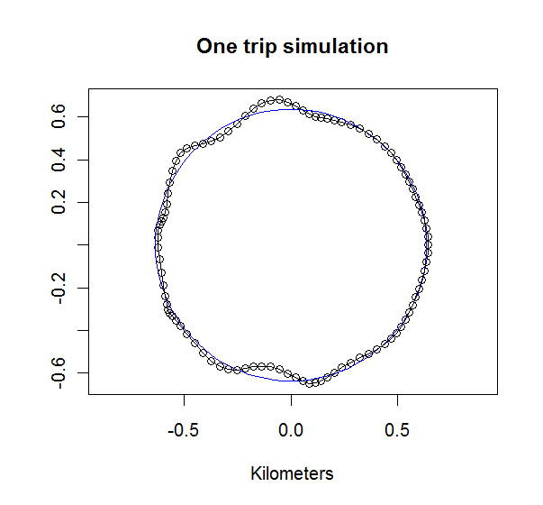
Therefore (a) we can expect some bias but (b) it may be difficult to predict. To illustrate this, I simulated a circular trip of 4 km, sampled to produce 100 segments (that would correspond to a point collection interval of around 15 seconds, but the actual number doesn't matter much). The simulation applied some quasi-realistic spatio-temporally correlated drift in the GPS readings with a root mean square error of about 45 m.

Here is a map of one simulated trip, showing the circular route in blue along with the GPS reading points:

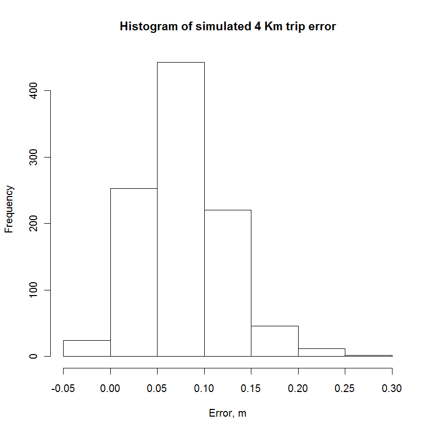
Here is a histogram of errors (differences between total GPS distance and 4 km) from 100 such simulations:

It is evident the error (in this case) is usually positive--the GPS measurement tends to overestimate this trip length--and averages around 100 meters. It is small, but comparable to the day-to-day variation in the trip readings.

This quasi-realistic analysis suggests it would be wise to

1. Calibrate the trip with an accurate distance measurement and

2. Record consistent point-to-point readings for each trip (even when running a little further to compensate for low readings).

With such data--it would likely require very little, maybe a couple of weeks' worth--you can begin answering questions about the accuracy and precision of the GPS measurement of trip length. Those questions are readily addressed by estimating means and confidence intervals for the means.

In the meantime, it seems it would be overkill to fret over variations of the order of 100 m or less, because it looks like these would reflect the precision of the measurement process rather than variations in the length of the trip.

Note that the accuracy and precision for a different route may change slightly, depending on the tortuosity of the route and even its location and time of day it tends to be run.

---

Here is the simulation (in R), for those who would like to modify it to conform to the characteristics of their routes and GPS units.

# Create a circular route of unit radius (to be rescaled later).
n <- 100
theta <- seq(0:n) / n * 2 * pi
x0 <- cos(theta)
y0 <- sin(theta)

# Compute some correlated perturbations to be added to the route.
cos.perturb = outer(theta, 1:10, FUN=function(t,k) cos(t*k))
sin.perturb = outer(theta, 1:10, FUN=function(t,k) cos(t*k))

# Simulate one trip, scaled by a given radius.
error <- function(radius=1) {
    x <- x0 + cos.perturb %*% rnorm(10, sd=.01) + sin.perturb %*% rnorm(10, sd=.01)
    y <- y0 + cos.perturb %*% rnorm(10, sd=.01) + sin.perturb %*% rnorm(10, sd=.01)
    dx <- diff(x)
    dy <- diff(y)
    distance <- sqrt(dx^2 + dy^2)

    # Return the trip error and the rmse deviation between GPS and true locations.
    radius * c((sum(distance) - 2 * pi), sqrt(mean((x-x0)^2 + (y-y0)^2)))
}

# Run a short simulation for a 4 Km route.
data <- replicate(10^3, error(4 / (2*pi)))

# Display the histogram of trip errors.
hist(data[1,], xlab="Error, m", main="Histogram of simulated 4 Km trip error")