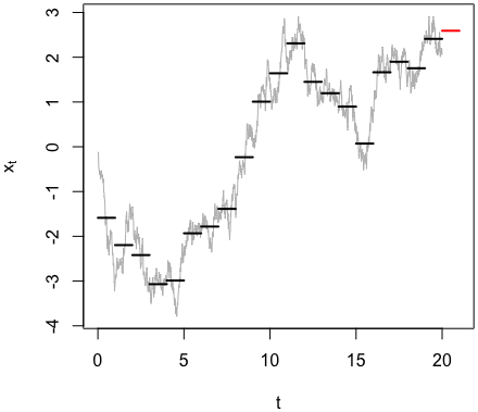
Let $B_t$ denote the state of the Brownian motion at each discrete time point $t=0,\pm 1,\pm 2,\dots$. Clearly, $B_t$ follows a random walk model
$$
(1-L)B_t = w_t \tag{1}
$$
where $L$ is the backshift operator and $w_t$ is Gaussian white noise with variance $\sigma^2$.
In-between two time points $t-1$ and $t$, conditional on $B(t-1)=B_{t-1}$ and $B(t)=B_t$, $B(t)$ is distributed as a Brownian bridge. It follows that the integral $x_t=\int_{t-1}^t B(t) dt$ of the bridge is normally distributed with conditional expectation $\frac12(B_t+B_{t-1})$. Using this formula for the covariance between $B(s)$ and $B(t)$, the conditional variance is
\begin{align}
\operatorname{Var}(x_t|B_t,B_{t-1})
&=\operatorname{Var}(x_1|B(1)=0,B(0)=0)
\\&=E\left(\int_0^1 B(t)dt\int_0^1 B(s)ds\right)
\\&=\int_0^1 \int_0^1 E(B(t)B(s))dsdt
\\&=2\int_0^1 \int_0^t \sigma^2 s(1-t) dsdt
\\&=\frac{\sigma^2}{12}.
\end{align}
In other words,
$$
x_t = \frac12(1+L)B_t + u_t, \tag{2}
$$
a moving average of the random walk $B_t$ plus white noise $u_t$ with variance $\sigma^2/12$.
Applying $(1-L)$ to both sides of (2) and using (1) yields
$$
(1-L)x_t = \frac12(1+L)w_t + (1-L)u_t. \tag{3}
$$
The right hand side of (3) is the sum of first order moving averages of two independent white noise processes and hence itself a first order moving average process that can be represented by $(1+\theta L)v_t$ where $v_t$ is another white noise process. Overall, $x_t$ thus satisfies a standard ARIMA(0,1,1) time series model
$$
(1-L)x_t = (1+\theta L)v_t. \tag{4}
$$
The moving average parameter $\theta$ and
the variance of $v_t$ in (4) can be determined by equating the autocovariance functions of the right hand sides of (3) and (4). This leads to
$$
\theta = 2-\sqrt{3}
$$
and
$$
\sigma_v^2 = \frac{2+\sqrt{3}}6 \sigma^2.
$$
From (4) it is apparent that the increments $\Delta x_t =(1-L)x_t$ are not independent but follow an MA(1) process. The correlation between $\Delta x_t$ and $\Delta x_{t-1}$ is $\theta/(1+\theta^2)=1/4$.
Forecasting of $x_{t+1}$ can now be done using standard methods. The infinite history forecast via the pure autoregressive AR$(\infty)$ representation of (4) is given by
$$
E(x_{t+1}|x_t,x_{t-1},\dots)=(1+\theta)(x_t - \theta x_{t-1} + \theta^2 x_{t-2} - \theta^3 x_{t-3} + \dots), \tag{5}
$$
a geometrically weighted average of past observations (red line segment in Figure below). Given that $\theta$ is quite small (0.2679), the forecast depends strongly only on the last few observations.

Alternatively, an exact finite history forecast can be computed via the state space representation of (4) using the Kalman filter but this will not differ much from (5) unless only a small number of observations are available.

