Validating a negative binomial glmm using glmmadmb in R

Question

In this post, I am seeking help to figure out how I can make sure the negative binomial glmm I'm running meets its model assumptions.

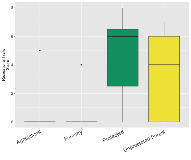
I am working with a dataset that I collected in the field documenting the presence of recreational trails along 28 streams, that were surrounded by four different land use type, and found in and around 7 different protected areas (i.e. National Parks). My original intention was to used a linear mixed model to assess the relationship between the "Recreational Trail Score" documented at each site and the different land use types, while accounting for the random effect of Park. Because the data has numerous (true) 0s, it was not possible to transform the data to attain a normal distribution. Consequently, I tried using a quasi-poisson glmm. This model was overdisperssed, so I decided to try using a negative bionomial model and am now seeking help to figure out if this model meets its assumptions or not. (I am suspicious that there is a a problem with the model because results don't seem in line with what I would expect given the data distribution shown in the box plot I've included below). Although I was able to locate a post that talks about validating glmms, its still unclear to me what exactly I need to check and how exactly I should check this to make sure the model is OK.

Below is R code that will allow you to reproduce the model I created. If anyone could provide feedback on: a) if this model is meeting its assumptions, and how exactly you are able to confirm that b) if its not, what would you recommend doing as a next step?

Create dataframe

RecreationalTrails<-c(5, 0, 0, 4, 7, 0, 0, 0, 6, 5, 0, 6, 6, 0, 0, 0, 0, 0, 
0, 0, 0, 0,4, 6, 8, 0, 0, 7)
 LandUse<-c("Protected", "Agricultural", "Forestry", "Unprotected Forest", 
 "Protected", "Agricultural", "Forestry", "Unprotected Forest",
   "Protected", "Agricultural", "Forestry", "Unprotected 
 Forest","Protected", "Agricultural", "Forestry", "Unprotected Forest",
   "Protected", "Agricultural", "Forestry", "Unprotected 
 Forest","Protected", "Agricultural", "Forestry", "Unprotected Forest",
   "Protected", "Agricultural", "Forestry", "Unprotected Forest")
Parc<-c("Monts Valin", "Monts Valin", "Monts Valin", "Monts Valin", "Fjords 
du Saguenay", "Fjords du Saguenay","Fjords du Saguenay",
"Fjords du Saguenay", "Hautes Gorges", "Hautes Gorges","Hautes 
Gorges","Hautes Gorges", "Grands Jardins", "Grands Jardins",
"Grands Jardins", "Grands Jardins", "Mont Tremblant", "Mont Tremblant", 
"Mont Tremblant", "Mont Tremblant", "Mauricie",
"Mauricie", "Mauricie", "Mauricie", "Jacques Cartier", "Jacques Cartier", 
"Jacques Cartier", "Jacques Cartier")
ESCombinedDataRE<-data.frame(c("LandUse", "Parc", "RecreationalTrails"))
ESCombinedDataRE <- data.frame(LandUse, Parc, RecreationalTrails)
names(ESCombinedDataRE) <- c("LandUse", "Parc", "RecreationalTrails")
ESCombinedDataRE

Visualize the data

RecTrails_boxplot<-ggplot(ESCombinedDataRE, aes(x=LandUse, y= 
RecreationalTrails, fill = LandUse))+
scale_fill_manual(values=c("#0072B2", "#56B4E9", "#009E73", "#F0E442"))+
geom_boxplot()+
theme_gray(base_size = 14)+
theme(legend.position="none",axis.text.x=element_text(size=18,angle=25, 
hjust=1, vjust=1), axis.title.y = element_text(size = 13),axis.text.y = 
element_text(size = 13),axis.title.x = element_text(size = 18))+
labs(x="",y="Recreational Trails\nScore") 
RecTrails_boxplot

Run glmer negative binomial model

 install.packages("glmmADMB", 
         repos=c("http://glmmadmb.r-forge.r-project.org/repos",
                 getOption("repos")),
         type="source")
 library(glmmADMB)

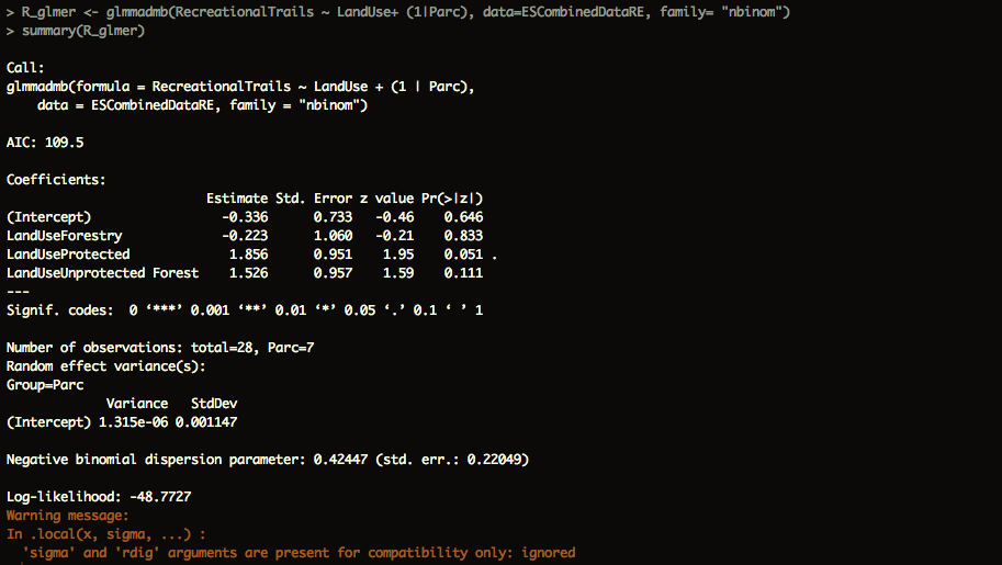
  R_glmer <- glmmadmb(RecreationalTrails ~ LandUse+ (1|Parc), 
  data=ESCombinedDataRE, family= "nbinom")

#Validate model (but how?!)
#Check overdispersion using this source code 
 https://rdrr.io/github/markushuff/PsychHelperFunctions/src/R/overdisp_fun.R
 overdisp_fun(R_glmer)

I believe that the overdispersion ratio of about 1 indicates that the model is not too over or under dispersed.

 #How else should I be checking that this model is meeting its assumptions? 

#Model output and results 
summary(R_glmer)

  #library(multcomp)
 summary(glht(R_glmer, linfct = mcp(LandUse = "Tukey")))
 #There appears to be no significant effect of land use on recreational 
 trails. This is very possible given the outliers and small sample size, but 
 I wanted to check that I've built this model correctly before trusting 
 it... 

Use this code to look at conditional and marginal R2 values

Answer 1

You can conveniently run residual diagnostics and overdispersion tests for GLMMs in DHARMa, see vignette here (disclaimer: I develop this package). Note: for neg binom, overdispersion is usually not a problem, but there are other issues to look at, see the DHARMa vignette.

At the moment, DHARMa supports neg.binom only for MASS and lme4 (current CRAN version of DHARMa), as well as glmmTMB (the latter with the development version of DHARMa, available here, will be on CRAN approximately June 2018).

I had originally planned to support glmmADMB as well, but have abandoned these plans due to reasons explained here. I suggests to all users that need functionalities that go beyond lme4 (btw, that doesn't see the case for you, why do you not use lme4?) to switch to glmmTMB.