Suppose you have two random variables such that
$$X_1 \sim N(\mu_1, \sigma^2_1) \text{ and } X_2 \sim N(\mu_2, \sigma^2_2).$$
If $X_1$ and $X_2$ are independent, then for any $a, b$
$$aX_1 + bX_2 \sim N(a \mu_1 + b\mu_2, a^2\sigma^2_1 + b^2\sigma^2_2). $$
This is by by properties of variance and expectation, and that the sum of two independent normals is a normal. The interpretation of this is not that the sampling distributions are being combined, but in fact that if you scale and add the random variables themselves, then you will end up with that sampling distribution.
If you realized $x_1$ for $X_1$ through one experiment and were to make $95\%$ confidence intervals for $\mu_1$ using this, the standard way to do this would give you
$$ x_1 \pm 1.96 \sqrt{\sigma^2_1}. $$
Now, similarly you ran a Binomial experiment, and over $n_1$ draws counted the number of successes. $\hat{p}_1$ is you average (proportion), and the sampling distribution for this is approximately
$$\hat{p}_1 \sim N\left(p_1, \dfrac{p_1(1-p_1)}{n_1} \right). $$
Similarly for the second experiment
$$\hat{p}_2 \sim N\left(p_2, \dfrac{p_2(1-p_2)}{n_2} \right). $$
If you now need to find a confidence interval for $p_1 - p_2$ you need its approximate sampling distribution. So you let $a = 1$ and $b = -1$.
$$\hat{p_1} - \hat{p_2} \sim N\left( p_1 - p_2, \dfrac{p_1(1-p_1)}{n_1} + \dfrac{p_2(1-p_2)}{n_2} \right).$$
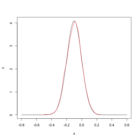
The interpretation of this sampling distribution is that is you get a sample of size $n_1 = 30$ from the first population and calculate $\hat{p}_1$ and get another sample from the second population of size $n_2 = 50$ and calculate $\hat{p_2}$; repeat this experiment 1000 times, and note down $\hat{p_1} - \hat{p_2}$, then these values will approximately following that sampling. distribution. I do this in the following R code.
set.seed(10)

## true values
p1 <- .2
p2 <- .3

n1 <- 30
n2 <- 50

diff_vector <- numeric(length = 1000)

for(i in 1:1000)
{
    X1 <- rbinom(1,n1, p1)
    phat1 <- X1/n1

    X2 <- rbinom(1,n2, p2)
    phat2 <- X2/n2

    diff_vector[i] <- phat1 - phat2
}

## parameters of the sampling distribution
diff_mean <- p1 - p2
diff_var <-  p1*(1-p1)/n1 + p2*(1-p2)/n2

x <- seq(-.8, .6, length = 1000)
y <- dnorm(x, mean = diff_mean, sd = sqrt(diff_var))

plot(x, y, type = "l")
lines(density(diff_vector), col = "red")
The plot below is the output you get. The black line is the sampling distribution expected, and the red line is the distribution obtained through the experiment. You see that they overlap. If you examine the code you will understand that I calculated the difference $\hat{p}_1 - \hat{p_2}$ over 1000 experiments, and then just plotted the density.

Using this sampling distribution you know that a standard $95\%$ confidence interval for $p_1 - p_2$ will be
$$\hat{p}_1 - \hat{p}_2 \pm 1.96 \sqrt{ \dfrac{p_1(1-p_1)}{n_1} + \dfrac{p_2(1-p_2)}{n_2}}.$$
This follows just as before.

