Are unbiased efficient estimators stochastically dominant over other (median) unbiased estimators?

Question

General description

Does an efficient estimator (which has sample variance equal to the Cramér–Rao bound) maximize the probability for being close to the true parameter $\theta$?

Say we compare the difference or absolute difference between the estimate and the true parameter $$\hat\Delta = \hat \theta - \theta$$

Is the distribution of $\hat\Delta$ for an efficient estimator stochastically dominant over the distribution of $\tilde\Delta$ for any other unbiased estimator?

---

Motivation

I am thinking about this because of the question Estimator that is optimal under all sensible loss (evaluation) functions where we can say that the unbiased best estimator with respect to one convex loss function is also unbiased best estimator with respect to another loss function (From Iosif Pinelis, 2015, A characterization of best unbiased estimators. arXiv preprint arXiv:1508.07636). The stochastic dominance for being close to the true parameter seems to be the similar to me (it is a sufficient condition, and a stronger statement).

---

More precise expressions

The question statement above is broad, e.g. what type of unbiasedness is considered and do we have the same distance metric for negative and positive differences?

Let's consider the following two cases$^\dagger$ to make the question less broad:

Conjecture 1: If $\hat \theta$ is an efficient mean and median-unbiased estimator. Then for any mean and median-unbiased estimator $\tilde \theta$ $$\text{if $x>0$ then } P[\hat\Delta \leq x] \geq P[\tilde\Delta \leq x] \\ \text{if $x<0$ then } P[\hat\Delta \geq x] \geq P[\tilde\Delta \geq x]$$ where $\hat \Delta = \hat \theta - \theta$ and $\tilde \Delta = \tilde \theta - \theta$

Conjecture 2: If $\hat \theta$ is an efficient mean-unbiased estimator. Then for any mean-unbiased estimator $\tilde \theta$ and $x>0$ $$ P[\vert \hat\Delta \vert \geq x] \leq P[\vert \tilde\Delta \vert \geq x] $$

• Are the above conjectures true?
• If the propositions are too strong, can we adapt them to make it work?

^{$\dagger$The second is related to the first but drops the restriction for median-unbiasedness (and then we need to take both sides together or otherwise te proposition would be false for any estimator that has a different median than the efficient estimator).}

---

Example, illustration:

Consider the estimation of the mean $\mu$ of the distribution of a population (that is assumed to be normal distributed) by (1) the sample median and (2) the sample mean.

In the case of a sample of size 5, and when the true distribution of the population is $N(0,1)$ this looks like

In the image we see that the folded CDF of the sample mean (which is an efficient estimator for $\mu$) is below the folded CDF of the sample median. The question is whether the folded CDF of the sample mean is below the folded CDF of any other unbiased estimator as well.

Alternatively, using the CDF instead of folded CDFs we can ask the question whether the CDF of a the mean maximizes the distance from 0.5 at every point. We know that $$\forall \hat \theta : |F_{mean}(\hat \theta)-0.5| \geq |F_{median}(\hat \theta)-0.5| $$

do we also have this when we replace $F_{median}(\hat \theta)$ for the distribution of any other mean and median-unbiased estimator?

Answer 1

Here is an experiment in a non-standard case, the location Cauchy problem, where non-standard means that there is no uniformly best unbiased estimator. Let us consider $(X_1,\ldots,X_N)$ a sample from a Cauchy $\mathcal{C}(\mu,1)$ distribution and the following four invariant estimators of $\mu$:

1. $\hat{\mu}_1= \text{median}(X_1,\ldots,X_N)=X_{(N/2)}$
2. $\hat{\mu}_2= \text{mean}(X_{(N/4)},\ldots,X_{(3N/4)})=\frac{2}{N}(X_{(N/4)}+\ldots+X_{(3N/4)})$
3. $\hat{\mu}_3=\mu^\text{MLE}$ which is efficient
4. $\hat{\mu}_4=\hat{\mu}_1+\frac{2}{N}\frac{\partial \ell}{\partial \mu}(\hat{\mu}_1)$

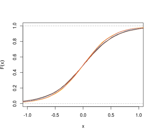
Then comparing the cdfs of the four estimators leads to this picture, where the cdfs of $\hat{\mu}_3$ (gold) and $\hat{\mu}_4$ (tomato) are comparable, and improving upon $\hat{\mu}_1$ (steelblue), itself improving upon $\hat{\mu}_2$ (sienna).

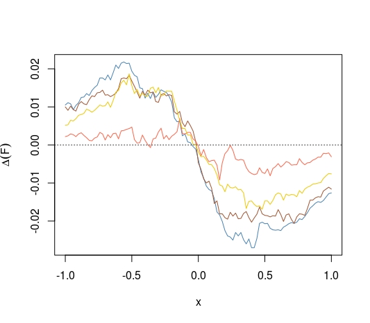
A representation of the differences to the empirical cdf of the MLE makes it clearer:

Here is the corresponding R code:

T=1e4
N=11
mlechy=function(x){
  return(optimize(function(theta) -sum(dcauchy(x, 
    location=theta, log=TRUE)),  c(-100,100))$minimum)
}
est=matrix(0,T,4)
for (t in 1:T){
cauc=sort(rcauchy(N))
est[t,1]=median(cauc)
est[t,2]=mean(cauc[4:8])
est[t,3]=mlechy(cauc)
est[t,4]=est[t,1]+(4/N)*sum((cauc-est[t,1])/(1+(cauc-est[t,1])^2))
}

plot(ecdf(est[,1]),col="steelblue",cex=.4,xlim=c(-1,1),main="",ylab="F(x)")
plot(ecdf(est[,2]),add=TRUE,col="sienna",cex=.4)
plot(ecdf(est[,3]),add=TRUE,col="gold",cex=.4)
plot(ecdf(est[,4]),add=TRUE,col="tomato",cex=.4)