Implementation of Shanken (1992) Adjustment for Fama MacBeth Asset Pricing Tests

Question

I am trying to implement an unconditional asset pricing test according to the Fama & MacBeth (1973) method. The calculation of the factor-loadings as average of monthly cross-sectional regressions are all set and working. A challenge I am facing is the implementation of a proper t-Stat. Originally I just the calculation based on Cochrane (2005): $$ \sigma^2(\lambda)=1/T^2*\sum \limits_{t=1}^T (\hat\lambda_t-\bar\lambda)^2 $$ This value I used in the t-Test: $$ tStat=\frac{\bar\lambda-0}{\sqrt{\sigma^2}} $$

As this calculation of the t-Stat does not contain a correction for the error in variables problem I looked for a Shanken (1992) adjustment on the standard error. Unfortunately many papers state, that they apply the Shanken adjustments to their t-Stats but do not include a calculation for it. I found a description for the implementation of a Shanken adjustment (http://lipas.uwasa.fi/~sjp/Teaching/eaptx/lectures/p5.pdf - slide 41 and following). This example also includes a sample implementation of the Shanken adjustment in Stata for a single cross-sectional regression. I used this example and transferred the calculations into Matlab code.

The problem now is that I am uncertain how the aggregation of periodic standard error calculations (following the Shanken adjustments) into one standard error for the t-test happens. With a single cross-section regression there is no aggregation of values - but for the periodical cross-section regression according to Fama & MacBeth I run monthly cross-sectional regressions.
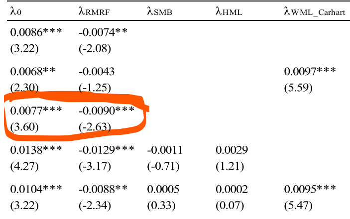
I implemented "my interpretation" of a Shanken adjustment in a 60 month rolling regression to reconcile the results of Artmann (2011: https://www.econstor.eu/bitstream/10419/70130/1/736358048.pdf page 36, table 8, panel F) who implemented a Shanken t-stat with Fama-MacBeth implementation.
I can reconcile the paper's factor loadings approximately but the calculated t-stats a far off.

Whereas the paper arrives at a t-stat of 3.6 for the intercept my t-stat is only 1.28. Hence I assume my implementation of the Shanken adjustment for the rolling beta estimation Fama-MacBeth procedure is faulty. My code works as follows:

% general calculation:
varianceOfDependent = cov(testAssetReturnData) ./ estimationPeriod;
factorCovariance = cov(factorData);

% ########################################################
% calculation for each cross-section regression:
% 1) variance calculation:
variance = (X'*X)^-1 * X' * varianceOfDependent * X * (X'*X)^-1; % variance estimate according to Cochrane, with X as Nxk matrix

% 2) calculate correctional factors
c =  regResult.beta(2:end) * factorCovariance^-1 * regResult.beta(2:end)'; % with regResult.beta(2:end) corresponding to the coefficient estimates for all factors (no intercept!)
modifiedFactorCovariance = [zeros(1,size(factorCovariance,2)+1); 

zeros(size(factorCovariance,2),1) factorCovariance];
    standardErrorsShanken = diag(sqrt(variance*(1+c) + modifiedFactorCovariance ./estimationPeriod))';
    tStatShanken = transpose(regResult.beta) ./ standardErrorsShanken; % transpose(regResult.beta) as lambda estimates of the period  

% ########################################################  
% Each tStatShanken is stored and the average is taken for each factor to arrive at the t-stat results

The implementation follows equation 41 of the linked paper:

Do you know how to properly implement the Shanken adjustments for the Fama-MacBeth approach?

Answer 1

I'm not an expert in this, but I think you used the wrong formula. Correct me if I'm wrong.

Summary of Shanken (1992)

Suppose that there are $k$ factors in the model. The number of time periods in months is $T$. In Shanken (1992), there are two formulae to correct the covariance matrix in the two theorems.

In Theorem 1, which applies to a cross-sectional regression of average returns, the formula is $$(1+c)\Omega+\Sigma_{\bar{F}}^*$$ where $\Omega=A\Sigma A^\top$ is the asymptotic covariance matrix of $\lambda$ in the cross-sectional regression and $c=\lambda^\top\Sigma_F^{-1}\lambda$. $\Sigma_{\bar{F}}^*$, a $(k+1)\times (k+1)$ matrix, is the bordered version of $\Sigma_F$ by augmenting the $k\times k$ matrix $\Sigma_F$ with a column and a row of zeros corresponding to the places of the intercept.

In Theorem 2, which applies to the Fama-MacBeth procedure with fixed beta estimated from the whole sample, the formula is $$(1+c)(\hat{W}-\Sigma_{\bar{F}}^*)+\Sigma_{\bar{F}}^*$$ where $\hat{W}$ is the asymptotic covariance matrix of $\lambda$ in the second step of the Fama-MacBeth procedure, i.e. $$\hat{W}=\frac{1}{T}\sum_{t=1}^T(\lambda_t-\bar{\lambda})(\lambda_t-\bar{\lambda})^\top$$ and $c=\lambda^\top\Sigma_F^{-1}\lambda$.

If we use a rolling-window of $y$ years to estimate beta prior to the Fama-MacBeth procedure, in the footnote of the appendix, Shanken (1992) shows that we should use the following $c^*$ in place of $c$ in the previous formula: $$c^*=\left[1-\frac{(y-1)(y+1)}{3yn}\right]c$$ where $T=12n$.

To summarize, if we want to use the Shanken's (1992) correction for the cross-sectional regression, we should use the formula in Theorem 1. If we want to use the correction for the Fama-MacBeth procedure, we should use the formula in Theorem 2.

Other evidence

There are two clues that the above summary is correct.

First, on Page 16 of the Shanken (1992) paper, the author makes an example to correct the standard error from Chen, Roll, and Ross (1986) that use the Fama-MacBeth procedure. In the formula $$(1+0.36)[(0.0318)^2-0.0561/324]+0.0561/324,$$ obviously we can see that the author uses the formula from Theorem 2.

Second, in a review paper, Goyal (2012) explicitly gives the formula for Shanken's (1992) correction applied to Fama-MacBeth regression in Eq. (33): $$T\cdot\mathrm{var}_{\mathrm{EIV}}(\hat{\lambda})=(1+c)[T\cdot\mathrm{var}(\hat{\lambda})-\Sigma_F]+\Sigma_F.$$

Finally, many people refer to Cochrane (2005). Actually if you read it carefully, the formula in Eq. (12.19) on page 240 for Shanken's correction is applied to the cross-sectional regression, as in Theorem 1. On page 249 when the author talks about the Fama-MacBeth procedure, he writes

If one is going to use them, it is a good idea to at least calculate the Shanken correction factors outlined above, and check that the corrections are not large.

However, no formula is provided here for the Fama-MacBeth regression. So I would rather trust the formula in Goyal (2012) for this case.

References:

Chen, N.F., Roll, R. and Ross, S.A., 1986. Economic Forces and the Stock Market. Journal of Business, 59(3), pp.383-403.

Cochrane, J.H., 2005. Asset pricing: Revised edition. Princeton university press.

Goyal, A., 2012. Empirical cross-sectional asset pricing: a survey. Financial Markets and Portfolio Management, 26(1), pp.3-38.

Shanken, J., 1992. On the Estimation of Beta-Pricing Models. Review of Financial Studies, 5(1), pp.1-33.

Answer 2

I think I got the answer of how to implement the adjustment:

Based on the variance of lambdas for the Fama/MacBeth calculation $$ \sigma_{OLS}^2(\lambda)=1/T^2*\sum \limits_{t=1}^T (\hat\lambda_t-\bar\lambda)^2 $$

I implemented the following adjustment: $$ \sigma_{Shanken}^2(\lambda)=\sigma_{OLS}^2(\lambda) * (1+c) + \frac{\tilde{\sum_F}}{T} $$ with: $$ c = \hat{\lambda} * cov(factors)^{-1}* \hat{\lambda}'$$ where:

• $$cov(factors)$$ is the variance-covariance matrix of assessed factors (which is an Nxk matrix for k-factors)
• $$\hat{\lambda}$$ is the lambda estimate vector resulting from the mean of periodic cross-sectional regression
• $$\tilde{\sum_F}$$ is the adjusted variance-covariance matrix from above with zeros in the first row and first column and the variance-covariance matrix in the right-bottom corner

When calculating a rolling-regression for the beta estimate the Shanken adjustments changes to c*: $$c^*=c*(1-\frac{1.6}{n})$$ with n as number of years in sample

!!! Please note that the adjustment factors changes if beta-estimation period deviates from a 60 month rolling beta approach !!!

Regards, Stonehenge