Is it possible to extract data points from moving average data?
In other words, if a set of data only has simple moving averages of the previous 30 points, is it possible to extract the original data points?
If so, how?
Is it possible to extract data points from moving average data?
In other words, if a set of data only has simple moving averages of the previous 30 points, is it possible to extract the original data points?
If so, how?
+1 to fabee's answer, which is complete. Just a note to translate it into R, based on the packages that I've found to do the operations at hand. In my case, I had data that is NOAA temperature forecasts on a three-month basis: Jan-Feb-Mar, Feb-Mar-Apr, Mar-Apr-May, etc, and I wanted to break it out into (approximate) monthly values, assuming that each three-month period's temperature is essentially an average.
library (Matrix)
library (matrixcalc)

# Feb-Mar-Apr through Nov-Dec-Jan temperature forecasts:

qtemps <- c(46.0, 56.4, 65.8, 73.4, 77.4, 76.2, 69.5, 60.1, 49.5, 41.2)

# Thus I need a 10x12 matrix, which is a band matrix but with the first
# and last rows removed so that each row contains 3 1's, for three months.
# Yeah, the as.matrix and all is a bit obfuscated, but the results of
# band are not what svd.inverse wants.

a <- as.matrix (band (matrix (1, nrow=12, ncol=12), -1, 1)[-c(1, 12),])
ai <- svd.inverse (a)

mtemps <- t(qtemps) %*% t(ai) * 3
Which works great for me. Thanks @fabee.
EDIT: OK, back-translating my R to Python, I get:
from numpy import *
from numpy.linalg import *

qtemps = transpose ([[46.0, 56.4, 65.8, 73.4, 77.4, 76.2, 69.5, 60.1, 49.5, 41.2]])

a = tril (ones ((12, 12)), 2) - tril (ones ((12, 12)), -1)
a = a[0:10,:]

ai = pinv (a)

mtemps = dot (ai, qtemps) * 3
(Which took a lot longer to debug than the R version. First because I'm not as familiar with Python as with R, but also because R is much more usable interactively.)
I try to put what whuber said into an answer. Let's say you have a large vector $\mathbf x$ with $n=2000$ entries. If you compute a moving average with a window of length $\ell=30$, you can write this as a vector matrix multiplication $\mathbf y = A\mathbf x$ of the vector $\mathbf x$ with the matrix
$$A=\frac{1}{30}\left(\begin{array}{cccccc} 1 & ... & 1 & 0 & ... & 0\\ 0 & 1 & ... & 1 & 0 & ...\\ \vdots & & \ddots & & & \vdots\\ 0 & ... & 1 & ... & 1 & 0\\ 0 & ... & 0 & 1 & ... & 1 \end{array}\right)$$
which has $30$ ones which are shifted through as you advance through the rows until the $30$ ones hit the end of the matrix. Here the averaged vector $\mathbf y$ has 1970 dimensions. The matrix has $1970$ rows and $2000$ columns. Therefore, it is not invertible.
If you are not familiar with matrices, think about it as a linear equation system: you are searching for variables $x_1,...,x_{2000}$ such that the average over the first thirty yields $y_1$, the average over the second thirty yields $y_2$ and so on.
The problem with the equation system (and the matrix) is that it has more unknowns than equations. Therefore, you cannot uniquely identify your unknowns $x_1,...,x_n$. The intuitive reason is that you loose dimensions while averaging, because the first thirty dimensions of $\mathbf x$ don't get a corresponding element in $\mathbf y$ since you cannot shift the averaging window outside of $\mathbf x$.
One way to make $A$ or, equivalently the equation system, solvable is to come up with $30$ more equations (or $30$ more rows for $A$) that provide additional information (are linearly independent to all other rows of $A$).
Another, maybe easier, way is to use the pseudoinverse $A^\dagger$ of $A$. This generates a vector $\mathbf z = A^\dagger\mathbf y$ which has the same dimension as $\mathbf x$ and which has the property that it minimizes the quadratic distance between $\mathbf y$ and $A\mathbf z$ (see wikipedia).
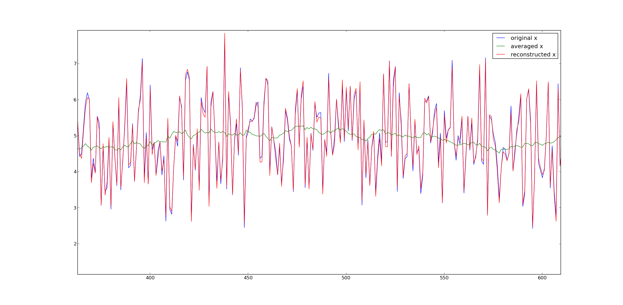
This seems to work quite well. Here is an example where I drew $2000$ examples from a Gaussian distribution, added five, averaged them, and reconstructed the $\mathbf x$ via the pseudoinverse.

Many numerical programs offer pseudo-inverses (e.g. Matlab, numpy in python, etc.).
Here would be the python code to generate the signals from my example:
from numpy import *
from numpy.linalg import *
from matplotlib.pyplot import *
# get A and its inverse
A = (tril(ones((2000,2000)),-1) - tril(ones((2000,2000)),-31))/30.
A = A[30:,:]
pA = pinv(A) #pseudo inverse

# get x
x = random.randn(2000) + 5
y = dot(A,x)

# reconstruct
x2 = dot(pA,y)

plot(x,label='original x')
plot(y,label='averaged x')
plot(x2,label='reconstructed x')
legend()
show()
Hope that helps.
This is very related with this question cumsum with shift of n I asked in SO.
I also answered in SO the same question as this one but it has been closed so I include here the answer again because I think is more focus in the software implementation than from the mathematical understanding (even though I think they are equivalent mathematically).
The question asked the same thing, how to reverse the moving average, a.k.a in pandas as rolling mean.
The code sample of the question:
import numpy as np
import pandas as pd
import matplotlib.pylab as plt
np.random.seed(100)
data = np.random.rand(200,3)

df = pd.DataFrame(data)
df.columns = ['a', 'b', 'y']

df['y_roll'] = df['y'].rolling(10).mean()
df['y_roll_predicted'] = df['y_roll'].apply(lambda x: x + np.random.rand()/20)
So, how to obtain df['y'] back from df['y_roll']? and apply the same method to df['y_roll_predicted']
With this function cumsum_shift(n) which you have to think of it as the inverse of the pandas/numpy method diff(periods = n), you can reverse the moving average up to constant if you don't have the initial values.
The definition of cumsum_shift(n) that generalizes the cumsum() which is this one with n = 1 (n is called shift in the code):
def cumsum_shift(s, shift = 1, init_values = [0]):
    s_cumsum = pd.Series(np.zeros(len(s)))
    for i in range(shift):
        s_cumsum.iloc[i] = init_values[i]
    for i in range(shift,len(s)):
        s_cumsum.iloc[i] = s_cumsum.iloc[i-shift] + s.iloc[i]
    return s_cumsum
Then assuming the size of the window is 10 win_size = 10 then if you multiply by 10 the diff'ed of the rolling mean and then "cumsum shift it" with a shift of 10, you obtain the original serie up to the intial values.
The code:
win_size = 10
s_diffed = win_size * df['y_roll'].diff()
df['y_unrolled'] = cumsum_shift(s=s_diffed, shift = win_size, init_values= df['y'].values[:win_size])
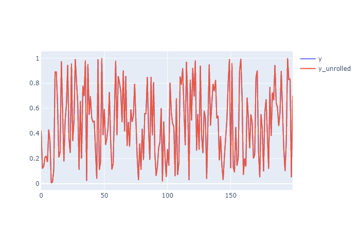
This code recovers exactly y from y_roll because you have the initial values.
You can see it plotting it (in my case with plotly) that y and y_unrolled are exactly the same (just the red one).

Now doing the same thing to y_roll_predicted to obtain y_predicted_unrolled.
Code:
win_size = 10
s_diffed = win_size * df['y_roll_predicted'].diff()
df['y_predicted_unrolled'] = cumsum_shift(s=s_diffed, shift = win_size, init_values= df['y'].values[:win_size])
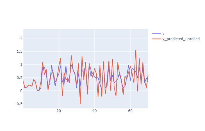
In this case the result are not exactly the same, notice how the initial values are from y and then y_roll_predicted incorporate noise to y_roll so the "unrolling" cannot recover exactly the original one.
Here a plot zoomed in in a smaller range to see it better:

Hope this can help somebody.
Gonzalo,
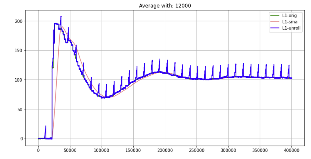
I'm using your cumsum_shift function in my large df (400,000 points) but I have problems when I change the win_size. Figure below is for win_size=12,000 and I can see some spikes at the end of each win_size. For my current problem I need to use win_size> 40,000. Do you have any idea of restriction of your function based on the win_size? Thanks in advance

fabee's answer was complete. I am just adding a generic function that can be used in Python that I've created and tested for my projects (with a sample code)
import numpy as np
import pandas as pd
import matplotlib.pyplot as plt


def reconstruct_orig(sm_x:np.ndarray, win_size:int=7):
    """reconstructing from original data

    Args:
        sm_x (np.ndarray): smoothed array (remove any NaN from the edge)
        win_size (int, optional): moving average window size. Defaults to 7.

    Returns:
        [type]: [description]
    """    '''
    '''
    arr_size = sm_x.shape[0]+win_size
    # get A and its inverse
    A = (np.tril(np.ones((arr_size,arr_size)),-1) - np.tril(np.ones((arr_size,arr_size)),-(win_size+1)))/win_size
    A = A[win_size:,:]
    pA = np.linalg.pinv(A) #pseudo inverse
    return np.dot(pA, sm_x)

if __name__=="__main__":
    # np.random.seed(1)
    nmax= 100
    t=np.linspace(0,10,num=nmax)
    raw_x = pd.Series(np.sin(t)+ 0.2*np.random.normal(0,1, size=nmax)) # create original data
    sm_x = raw_x.rolling(7, center=False).mean().dropna() # smooth data
    re_x = reconstruct_orig(sm_x, win_size=7)          # reconstruct data

    plt.plot(raw_x,'x',label='original x')
    plt.plot(sm_x,label='averaged x')
    plt.plot(re_x,'.', label='reconstructed x')
    plt.legend()
    plt.show()