Suppose you want to estimate the average height of students at a university. Roughly speaking heights
are normally distributed and have a standard deviation
of about 3.5 inches. Almost all the probability in
a normal distribution is within about 3 standard deviations on either side of the mean. So, whatever
the mean is students heights will mainly fit into
an interval of width 6 standard deviations or $6(3.5)=21$ inches. That seems about right.
Now suppose you sample one student at random from the student body and measure his or her height. This student might be near average in height, unusually short, or unusually tall. In fact, it would be no surprise if that one height were
as much as 7 or 8 inches shorter or taller than the university mean.
If I randomly sample a few students, it seems unlikely
that they will all be very short or very tall. Maybe
a few short ones, a few tall ones, and a few just about average. And if we take their average heights the tall and short ones would 'average out'. So the average
of a few heights must give a better estimate of the average
height in the university than does just one individual.
The idea is that averages are more stable than
individual values. I don't know how to give an intuitive
argument that the standard deviation of an average decreases at a rate obtained by dividing by $\sqrt{n}.$
(Partly, a formal proof of that depends on using the standard
deviation as a measure of variability, and most beginners don't have much intuition about standard deviations to use as a basis of an intuitive argument.)
A simulation might help. Suppose that the true distribution of heights at this university is normal
with mean $\mu = 58$ inches and standard deviation $\sigma = 3.5$ inches. I can use R statistical
software to sample 100 students from such a population.
The sample standard deviation is about 3.5 for 100 individual students.
set.seed(1234)
x = rnorm(100, 58, 3.5)
mean(x);  sd(x)
[1] 57.45133
[1] 3.515419
If I had the patience to take 100 thousand samples
of size $n = 16,$ I could find the standard deviation
of each sample. According to your fourmula, these standard deviations should
be something like $3.5/\sqrt{16} = 0.875.$
In a few seconds, R can do this huge job of taking the samples, summarizing the results of each sample, and giving
an overview of the results. The standard deviation
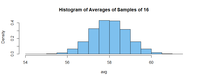
of the averages of $n = 16$ students turn out to be
about 0.87, which agrees pretty well with the formula.
set.seed(814)
avg = replicate( 10000,  mean(rnorm(16, 58, 3.5)) )
sd(avg)
[1] 0.8692906
Here is a histogram of the averages of samples of size 16. Using the mean of a sample of 16 students is very likely to give me an estimate of $\mu$ that is is within two inches of the correct answer. A sample of 64 students (4 times as big) should get me an estimate correct to the nearest inch.


