This isn't a direct answer to your question, but it does illustrate
what information you need to input to a 'power and sample size' procedure
to get the required sample size.
Let's suppose the current number of "energy units" per day for
30,000 households is $100.$ With new technology you expect energy consumption
per household to be normally distributed with mean $\mu < 100$ with
$\sigma = 20.$ You hope to have power 90% of detecting decrease of as
much as $5$ energy units. So if the particular alternative
$H_a: \mu = 95$ is true you want the rejection probability to be $0.9 = 90\%.$
To be sure, some of this "information" may be unknown and speculative,
but all of the above is necessary input. (You can experiment
with slight variations of the input to see the effect of the output.)
Here is output from a recent release of Minitab to illustrate:
Power and Sample Size

1-Sample t Test

Testing mean = null (versus < null)
Calculating power for mean = null + difference
α = 0.05  Assumed standard deviation = 20

            Sample  Target
Difference    Size   Power  Actual Power
        -5     139     0.9      0.901145
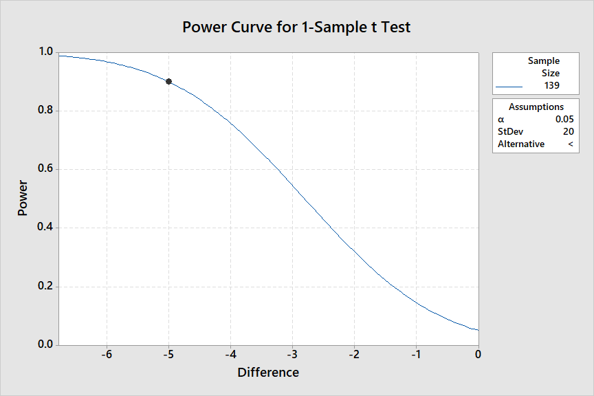
So in this hypothetical scenario you would need a sample size of $n = 139$
to get the desired power. The following graph shows power for detecting
a decrease of $5$---along with other possible decreases.

Under my assumptions, it seems feasible to install the new technology in about 140 houses and
to do a one-sample t test of the results $H_0: \mu=100$ vs. $H_a: \mu < 100$ at the 5% level.
Notes: (1) For normal data, such computations use a non-central t distribution with degrees of freedom $n - 1$ and a non-centrality parameter that depends of desired power, size of difference to detect, and anticipated population SD for the $n$ observations.
The crucial fact is that $n = 129$ observations suffice to give
90% power of a difference that is $5/20 = 1/4$ as large as the anticipated SD.
You can search
this site, and the Internet for technical explanations at your level. This recent Q&A may be helpful.
(2) Many statistical computer programs have 'power and sample size' procedures. There is a library in R with such procedures for a variety
of types of tests. There are online sites for power and sample size
computations, but not all of those are reliable.
(3) In R, the probability functions dt, pt, and so on have a
(seldom used) parameter 'ncp` for the non-centrality parameter.
Simulation in R: With 100,000 iterations, one can expect about two-place
accuracy. So the simulation is in essential agreement with the Minitab output.
set.seed(1121)
pv = replicate(10^5, t.test(rnorm(139, 95, 20), mu=100, alt="less")$p.val)
mean(pv <= 0.05)
[1] 0.89914

