How to choose between Pooled and Satterthwaite methods in t test for 2 small samples with marginally different variances?

Question

I compare means (or medians) of the numeric variable X for two groups composed of 6 and 18 subjects (using SAS). How do I choose between Pooled and Satterthwaite methods if the F-test for Equality of Variances is 0,046, i.e., marginally significant while using the Pooled method the p-value is 0.056 and in the case of Satterthwaite it is 0.007, i.e. they are very different.

And is the t-test the right test to use with this data taking into consideration that Kolmogorov-Smirnov and other criteria for normality of the distribution of the of 6 subjects in the first group show p-values around 0.04?

I also performed the Mann-Whitney U-test and it gave p=0.07 (Wilcoxon) and p=0.053 (Kruskal). But the shape of histograms for two groups looks quite different, so my concern is that it means that one of the assumptions of Mann-Whitney U test is also violated. However, may I conclude from all these tests that the p-value is above 0.5? Or is it possible that the p-value is actually < 0.05?

The data is the following.

Group 1: 0.35894, 0.38882, 0.36004, 0.37289, 0.54223, 0.50994.
Group 2: 0.44332, 0.82616, 0.65995, 0.30866, 0.36630, 0.31708, 0.83976, 0.75948, 0.45998, 0.62960, 0.87457, 0.57932, 0.68573, 0.54461, 0.76902, 0.39784, 0.99413, 0.38794.

Answer 1

Thanks for providing the data. I will jump ahead and say that I'd be uncomfortable saying, at the 5% level, that the two samples come from populations with different locations. At the 6% level, Yes. If you intended a one-sided test that population 2 is centered above population 1, Yes at the 5% level.

So this is a case where there is not enough data to claim significant difference of a two-sided test at the 5% level. The main difficulties are that x1 is so small and has four "low" values along with two "high" ones: the location of the center of its population is unclear.

In such situations, the principled course of action is no admit that there is not quite enough data for a convincing result. If the issue at hand is of great importance, perhaps there is enough evidence of a possible difference to warrant a second study, perhaps with more observations.

A less-principled course of action is to 'shop around' among borderline plausible tests until you find one that gives a P-value barely below 5%. This is a path that has led to many published "false discoveries" that no one has been able to replicate with an appropriately powered subsequent study.

x1 =  c(0.35894, 0.38882, 0.36004, 0.37289, 0.54223, 0.50994)
x2 =  c(0.44332, 0.82616, 0.65995, 0.30866, 0.36630, 0.31708, 0.83976, 0.75948, 0.45998,
        0.62960, 0.87457, 0.57932, 0.68573, 0.54461, 0.76902, 0.39784, 0.99413, 0.38794)

Examining the data, I notice that even though x1 has only six observations, it fails a Shapiro-Wilk test of normality with P-value around 3.6%.

shapiro.test(x1)$p.val 
[1] 0.03581921

One should be wary of using t tests (pooled or Welch) with such a small non-normal dataset. That might suggest using a nonparametric 2-sample Wilcoxon (rank sum) test. But an assumption of a straightforward use of this test is that the two samples have similar 'shapes', which includes having roughly equal variances. However, your x1 obviously has a much smaller variance than does you x2.

stripchart(list(x1,x2), ylim=c(.5,.2.5), pch="|")

So we can use the Wilcoxon signed rank test to check for 'stochastic dominance' but not specifically for unequal medians. At the 6% level one can say that one population dominates the other. At the 3% level one can say that x2 has significantly larger values than x1.

wilcox.test(x1,x2)$p.val
[1] 0.05585604

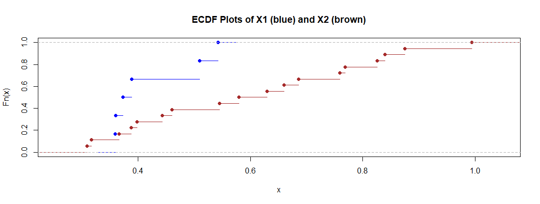
This dominance is illustrated by empirical CDFs (ECDFs) of the two samples: The plot for x2 lies (mostly) below and to the right of the plot for x1.

plot(ecdf(x2), col="brown", main="ECDF Plots of X1 (blue) and X2 (brown)")
 lines(ecdf(x1), col="blue")

Other than for 'P-hacking', I find no reason to use a Welch two-sample t test, on account of the (aggressive) non-normality of x, mentioned above. However, for full disclosure, here are its (significant) results:

t.test(x1,x2)

        Welch Two Sample t-test

data:  x1 and x2
t = -3.0067, df = 21.159, p-value = 0.00668
alternative hypothesis: 
  true difference in means is not equal to 0
95 percent confidence interval:
 -0.30489818 -0.05564293
sample estimates:
mean of x mean of y 
0.4221433 0.6024139 

If one tries to argue that the population that produce x1 might be normal after all, then the issue is whether it's normal with mean around 3.7 or around 5.2 (and with what variance?), and what results those scenarios might yield. We simply don't know much about population 1.

It would be difficult to argue that any one analysis of such a dataset is the correct one, and there are enough issues with your data that others may recommend alternative analyses. Possibly, different analyses may appear on this page. However, I would not want to claim a significant difference between the two populations at the 5% level based on your data.

Answer 2

It is my belief that the assumption of equal variance is pretty much always wrong, so use the Satterthwaite method unless you have reason to believe the two groups have equal variance (such as performing a simulation where you know the variance). The fact that the default in R is to use the Satterthwaite approximation makes me confident that my approach is a good one. Watch out for this in the software you use, because R might be unusual in this way (though I think they made the right decision).