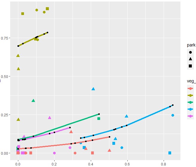
I have a beta regression model in R, have generated predicted (fitted) values based on my data, and plotted lines of those fitted values on a scatter plot of the actual data. I'm most used to GLMMs, and, at least in practice, have been thinking about the beta regression in a similar way.
However, the fitted values for this additive-only fixed-effects model are not creating a straight line, nor are the slopes the same between groups. I was expecting the fitted values to show the same slope, with different intercepts per group. Was that the wrong expectation? Or does this suggest there is an issue with either my data or implementation?

About the data:
y = a 0 to 1 proportion value of [# individuals in an experiment plot on a vegetation type]/[# individuals found across vegetation types within that plot]
x_coverage = a 0 to 1 proportion value of [amount of a vegetation type in a plot]/[total amount of vegetation measured in that plot]
x_type = a categorical factor of the type of vegetation a measurement was taken on
9 plots in the study (study site was once considered as a random variable, but AICc has me leaving it out), a section of the data:
| site | plot | x_type | x_coverage | y | fit |
|---|---|---|---|---|---|
| S1 | 1 | B | 0.143312327 | 0.916667 | 0.77496105 |
| S1 | 2 | B | 0.102556653 | 0.931034 | 0.75413317 |
| S1 | 3 | B | 0.107069321 | 0.738462 | 0.756502 |
| S2 | 4 | B | 0.001628412 | 0.215385 | 0.69722273 |
| S3 | 5 | B | 0 | 0.631579 | 0.69624543 |
| S3 | 6 | B | 0.002018163 | 0.545455 | 0.69745638 |
| S4 | 7 | B | 0.161420819 | 0.938776 | 0.78380402 |
| S4 | 8 | B | 0.09705228 | 0.741176 | 0.7512228 |
| S4 | 9 | B | 0.02603157 | 0.90625 | 0.711652 |
| S1 | 1 | P | 0 | 0.016667 | 0.08769793 |
| S1 | 2 | P | 0 | 0 | 0.08769793 |
| S1 | 3 | P | 0 | 0.015385 | 0.08769793 |
| S2 | 4 | P | 0.083824442 | 0.338462 | 0.10871038 |
| S3 | 5 | P | 0 | 0 | 0.08769793 |
| S3 | 6 | P | 0 | 0 | 0.08769793 |
| S4 | 7 | P | 0 | 0.020408 | 0.08769793 |
| S4 | 8 | P | 0.44368743 | 0.223529 | 0.2531569 |
| S4 | 9 | P | 0 | 0.03125 | 0.08769793 |
| S1 | 1 | T | 0.343765489 | 0.066667 | 0.09710628 |
| S1 | 2 | T | 0.570017432 | 0.034483 | 0.16978323 |
| S1 | 3 | T | 0.848919012 | 0.246154 | 0.31109899 |
| S2 | 4 | T | 0.412763648 | 0.415385 | 0.11569752 |
| S3 | 5 | T | 0.595125254 | 0.236842 | 0.18007354 |
| S3 | 6 | T | 0.534252719 | 0.090909 | 0.15594049 |
| S4 | 7 | T | 0.83374445 | 0 | 0.30193773 |
| S4 | 8 | T | 0.364015573 | 0.035294 | 0.10226738 |
| S4 | 9 | T | 0.52603157 | 0.0625 | 0.1528916 |
About the model:
gamlss(data=newbyplotvegpred, y ~ x_coverage + x_type, family="BEINF0")
Used a zero-inflated hurdle model version of the beta regression (BEINF0), as y contains zero-values (which are fairly believable as real zeros given our methods). Transforming the data and using plain BE changed the fitted values, but not the fact that slopes varied by vegetation type. Double checks with package betareg and glmmtmb give essentially the same results.
Predicted values were generated by predict(MODEL, type = "response). Not specifying type, defaults to values scaled to the predictor vars (as I understand it), and indeed produce same-slope lines. But truly wacky intercepts.
Fitted values put into ggplot with geom_point and geom_line (< 10 data points, catches an error for geom_smooth).
Any thoughts on what's up with these regression lines I'm plotting. The summary(MODEL) output is sensible, and I feel like that aspect of the our approach has been reasonable. Thank you!
