comparing distribution of values to a fixed estimate

Question

This is obviously a partial duplicate of statistical test to compare a distribution of values versus a fixed number but I hope with greater explanation of what I'm trying to do to get a more defined answer

short question: I have a distribution of responses to task a and I want to compare these to the fit of a logistic regression of responses to a very similar task b. I obviously have the individual responses to a so can calculate the mean, standard deviation, sem of the dependent variable, etc. For task b, I only have the fitted estimate of dependent variable and the error of this fit. It feels I want to use some t-statistic but I wanted to check if this is right and also get a better understanding of the thought process to get there.

longer question: It might be easier if I make up a relevant example and also give synthetic data.

Let's say I am interested in finding out the value of two bars of chocolate (one low quality, one high quality) to my friend. For simplicity, I'll call him F.

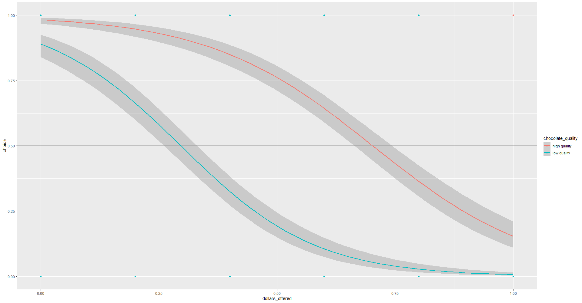
At first I give him repeated choices between the chocolates and some dollar amount (between 0 and $1 in 20cent increments). F's choices are noisy and so over choices we get a nice psychometric curve on choices

# ground truth
value_low_quality <- 0.3
value_high_quality <- 0.7
n <- 100

#synthetic choice data
choice_data <- seq(0, 1, 0.2) %>%
  #generate distributions
  data.frame(x = .,
             y1 = 1-pnorm(., value_low_quality, 0.25),
             y2 = 1-pnorm(., value_high_quality, 0.3)) %>%
  #melt data
  gather("group", "percent_choice_chocolate", - x) %>%
  mutate(chocolate_quality = case_when(
    group == "y1" ~ "low quality",
    group == "y2" ~ "high quality"
  )) %>%
  rename(dollars_offered = x) %>%
  select(chocolate_quality, dollars_offered, percent_choice_chocolate) %>%
  #make choices into individual trials
  group_by(chocolate_quality, dollars_offered) %>%
  group_split() %>%
  map_df(function(d) {
    trial_data <- d %>% slice(rep(1, each = n))
    n_choose_choc = round(d$percent_choice_chocolate * n)
    
    choices <- c(rep(1, n_choose_choc), rep(0, n - n_choose_choc))
    trial_data$choice <- choices
    return(trial_data)
  })

and to plot these choices as a binary response with a fitted curve

binomial_smooth <- function(...) {
  geom_smooth(method = "glm", method.args = list(family = "binomial"), ...)
}

p1 <- ggplot(choice_data, aes(x = dollars_offered, y = choice, colour = chocolate_quality)) +
  geom_hline(yintercept = 0.5) +
  geom_point() +
  binomial_smooth()

we can infer the value of each chocolate as the dollar amount for which F chooses either the chocolate or the dollars 50% of the time (line).

I can calculate this point using the MASS package p.dose function, here I've pulled the raw code out of these just in case my understanding of what this function does is incorrect.

choice_values <- map_df(c("low quality", "high quality"), function(q, d) {
  #filter
  d <- d %>%
    filter(chocolate_quality == q)
  #model
  model <- glm(choice ~ dollars_offered, family = "binomial", data = d)
  
  #care about the x value about choice p = 0.5
  p = 0.5

  eta <- family(model)$linkfun(p)
  coef <- coef(model)
  expected_value_x <- (eta - coef[1L])/coef[2L]
  pd <-  -cbind(1, expected_value_x)/coef[2L]
  SE <- sqrt(((pd %*% vcov(model)) * pd) %*% c(1, 1))
  
  return(data.frame(chocolate_quality = q, inferred_value = expected_value_x, se = SE))
}, d = choice_data)

choice_values

chocolate_quality  inferred_value  se
low quality        0.2966116       0.01751509
high quality       0.7025652       0.02005506

So that is all fine and good and I have my point estimate of the value of each chocolate.

The next day I'm still curious so I ask F to do a further 200 trials where on each he states how much he would be willing to pay (WTP) for each bar of chocolate

#more synthetic data
wtp_data <- data.frame(
  chocolate_quality = rep(c("low quality", "high quality"), each = n),
  bids = c(rnorm(n, value_low_quality, 0.3), rnorm(n, value_high_quality - 0.35*value_high_quality, 0.2))
)

I've added a deviation for the bids for the high value chocolate so we have one group where values/distributions from both tasks are effectively equal (h0 - no difference in estimates) and one where the values/distributions are unequal (h1), or at least approaching h1. The actual result here doesn't matter.

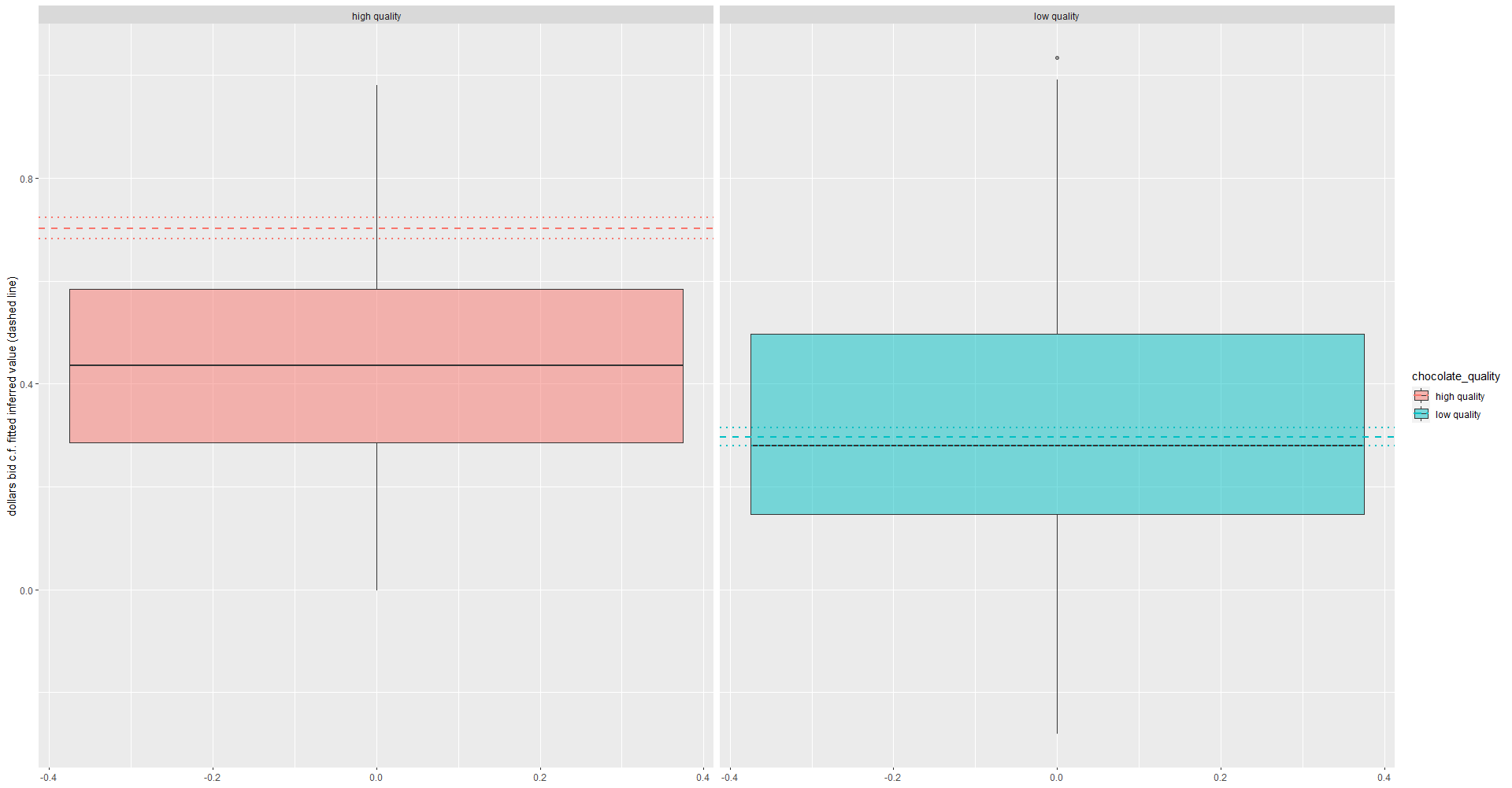
If I then plot the values I can see the how these estimates of values compare

p2 <- ggplot(wtp_data, aes(y = bids, fill = chocolate_quality)) +
  geom_boxplot(alpha = 0.5) +
  geom_hline(data = choice_values, aes(yintercept = inferred_value, colour = chocolate_quality), linetype = "dashed", size = 1) +
  geom_hline(data = choice_values, aes(yintercept = inferred_value + sem, colour = chocolate_quality), linetype = "dotted", size = 1) +
  geom_hline(data = choice_values, aes(yintercept = inferred_value - sem, colour = chocolate_quality), linetype = "dotted", size = 1) +
  facet_wrap(~chocolate_quality) +
  labs(y = "dollars bid c.f. fitted inferred value (dashed line)")

And we can see the similarity in estimates for the low quality chocolate and the deviation for the high quality chocolate. But I'm not sure how to statistically examine these differences.

Answer 1

First, Kvam & Busemeyer (2020) have recently published a Psych Review paper on this topic which you may find useful (preprint here).

Kvam, P. D., & Busemeyer, J. R. (2020). A distributional and dynamic theory of pricing and preference. Psychological Review, 127(6), 1053–1078. https://doi.org/10.1037/rev0000215

I can see two principled approaches you could take here.

Bootstrap

Let's call the indifference point calculated from the choices $\mu_c$, the average valuation $\mu_v$, and the difference between the two $\delta \mu$. You already know how to calculate these estimates from your $N_c$ and $N_v$ data points.

A bootstrap estimate of $\delta \mu$ can be obtained by a) drawing $N_c$ samples with replacement from the choice data, and $N_v$ with replacement from the valuation data, b) calculating $\mu_c$, $\mu_v$, and $\delta \mu$ for the resampled data, and c) repeating this procedure 1000 times or so, producing a bootstrap distribution for $\delta \mu$.

Full Probability Model

Alternatively, you can set up a statistical model that specifies the likelihood of observing your data under different sets of parameter values. A general purpose way of using doing this is with a probablistic programming language such as Stan, where you would also specify prior distributions for your parameters, and obtain samples from the posterior distribution, given your data.

A sensible approach here is to assume your valuation data come from a normal distribution with mean $\mu_v$ and SD $\sigma_v^2$, while your choice data come from a binomial probit distribution: they choose the cash if it exceeds a threshold $x$, where $x \sim \text{Normal}(\mu_c, \sigma_c^2)$ varies randomly from trial to trial.