My goal is to use a linear mixed effects model to test whether diurnality can be predicted by an animal's reproductive code, the season, and the fate of the animal at the end of the study period. All predictors are categorical, and the response variable is a continuous variable bounded between -1 and 1. Diurnality measures whether an animal is more active during the day or at night, and is calculated by: diurnality = (daysl/dayn - nightsl/nightn)/(daysl/dayn + nightsl/nightn), where sl is the distance travelled during the day or night (continuous) and n is the number of hours we have data for (integer) - therefore, each term is a movement rate. Data is summarized below; I cannot share it because 1) it is very large and 2) it is not owned by me.
summary(diurnalitydata)
     name               year               daysl              dayn
 Length:56202       Length:56202       Min.   :    0.9   Min.   : 1.00
 Class :character   Class :character   1st Qu.: 1938.9   1st Qu.:10.00
 Mode  :character   Mode  :character   Median : 4152.0   Median :13.00
                                       Mean   : 5316.4   Mean   :12.74
                                       3rd Qu.: 7329.3   3rd Qu.:15.00
                                       Max.   :44245.9   Max.   :18.00
    nightsl            nightn         diurnality
 Min.   :    0.0   Min.   : 1.000   Min.   :-0.9956
 1st Qu.:  310.4   1st Qu.: 6.000   1st Qu.: 0.1399
 Median :  746.7   Median : 7.000   Median : 0.4628
 Mean   : 1513.4   Mean   : 7.831   Mean   : 0.3844
 3rd Qu.: 1733.3   3rd Qu.:10.000   3rd Qu.: 0.7100
 Max.   :29125.4   Max.   :16.000   Max.   : 1.0000
              season       Code          fate
 hypophagia      :15122   FAd:16133   alive:48420
 earlyhyperphagia:18953   FSA: 8272   dead : 7782
 latehyperphagia :22127   FWC:15174
                          MAd:11512
                          MSA: 5111
The response variable is continuous, bounded between -1 and 1, and left skewed
I used a linear mixed effects model (lmertest) to fit this model:
> Diurnalitylmer <- lmer(diurnality ~ fate + Code + season  + (1|name/year), data=diurnalitydata)
> summary(Diurnalitylmer)
Linear mixed model fit by REML. t-tests use Satterthwaite's method ['lmerModLmerTest']
Formula: diurnality ~ fate + Code + season + (1 | name/year)
   Data: diurnalitydata

REML criterion at convergence: 48671.3

Scaled residuals:
    Min      1Q  Median      3Q     Max
-4.1855 -0.6048  0.1607  0.7283  3.2634

Random effects:
 Groups    Name        Variance Std.Dev.
 year:name (Intercept) 0.01686  0.1298
 name      (Intercept) 0.01772  0.1331
 Residual              0.13719  0.3704
Number of obs: 56202, groups:  year:name, 208; name, 111

Fixed effects:
                         Estimate Std. Error         df t value Pr(>|t|)
(Intercept)             4.220e-01  2.435e-02  1.016e+02  17.332  < 2e-16 ***
fatedead                5.043e-02  4.294e-02  1.112e+02   1.174  0.24275
CodeFSA                 3.268e-04  7.171e-03  5.311e+04   0.046  0.96365
CodeFWC                 6.830e-04  5.250e-03  5.588e+04   0.130  0.89650
CodeMAd                -9.321e-02  3.322e-02  1.117e+02  -2.805  0.00593 **
CodeMSA                -8.652e-02  3.416e-02  1.245e+02  -2.533  0.01255 *
seasonearlyhyperphagia -2.339e-02  4.442e-03  5.496e+04  -5.267  1.4e-07 ***
seasonlatehyperphagia  -4.458e-02  4.628e-03  5.077e+04  -9.633  < 2e-16 ***
---
Signif. codes:  0 ‘***’ 0.001 ‘**’ 0.01 ‘*’ 0.05 ‘.’ 0.1 ‘ ’ 1

Correlation of Fixed Effects:
            (Intr) fatedd CodFSA CodFWC CodMAd CodMSA ssnrly
fatedead    -0.214
CodeFSA     -0.102 -0.017
CodeFWC     -0.089 -0.008  0.313
CodeMAd     -0.662 -0.128  0.080  0.067
CodeMSA     -0.638 -0.154  0.078  0.065  0.918
ssnrlyhyprp -0.108  0.006  0.000  0.000  0.008  0.007
ssnlthyprph -0.117  0.002  0.000  0.001  0.016  0.014  0.626
> plot(Diurnalitylmer)
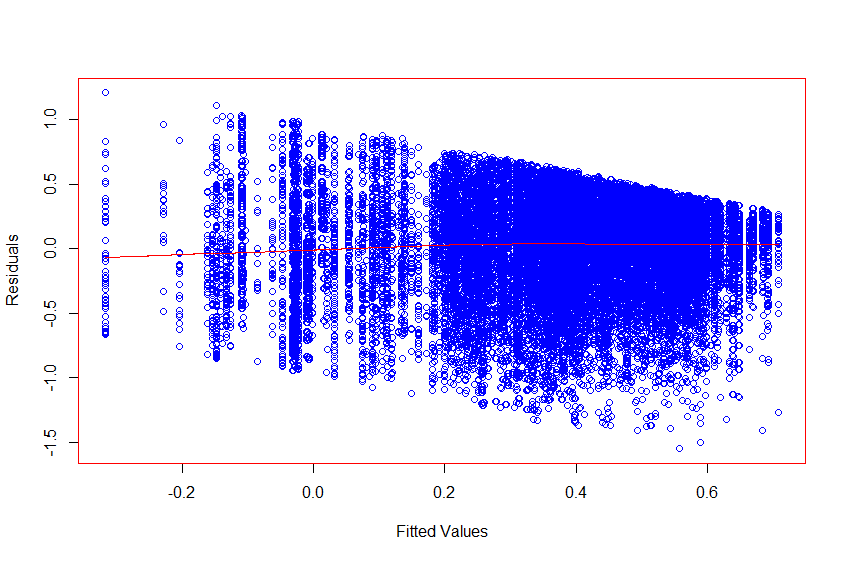
The residuals look like this; loess line is in red:
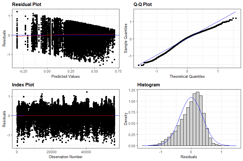
More diagnostics from ggResidpanel:
What I want to know is: is there a transformation, or model variation that I can use that can help me to meet the lme assumptions, or is lme out of the question for this data?
There are several similar questions on Stack Exchange - I've probably read through 20. For example: decreasing trend in residual plot for linear regression
However, for most of these - at least the ones with accepted answers - the response variable was discrete. Also, my "lines" are vertical, not following the trend - which I'm guessing has to do with my categorical predictors. I know that the bounds in my residuals are because the response is bounded, but I still don't quite understand why it's decreasing or what to do about it. Most of the recommendations for using a glmm with a different distribution require positive data (e.g. Poisson, Gamma).
My question seems very similar to this one: How to handle bounded [0,1] dependent variable that causes one to fail heteroscedasticity It is recommended to use a binomial response, but in this case, the denominator in the response is discrete, whereas mine is not (although the "n" is), and I'm not getting the parallel decreasing lines. Another suggestion is to use a beta distribution, but I believe that is for [0,1] data and it sounds like it would be a problem for my data because my data goes right up against the bounds.
I've been struggling with this for a couple days now, and any help would be greatly appreciated! I'd like to keep my methods pretty similar because my other analyses are using lme and I'd like them to be comparable - but if that's not possible I'd be happy to know and move on. Thanks!


