1
$\begingroup$

Say you have a null hypothesis of p = .6 and an alternative hypothesis of p < .6 and you decide to run the test at an α = .05. You get a P-Value of .03 and therefore reject the null hypothesis since P < .05.

From what I have seen, the chance of getting a type 1 error is equal to the alpha level, so 5% in this case. However, if I used the exact same data set, but tested at α = .10, now the chance of getting a type 1 error would be 10%? Intuitively, the chance of getting a false positive should be a set value, whatever it may be.

So I guess my question is why would the chance of a false positive/type 1 error be 5% in the 1st example and not 3%?

$\endgroup$
1
  • $\begingroup$ You are confusing two things: (a) Fixed $\alpha = P(\mathrm{Rej} H_0|H_0 \mathrm{true}).$ which is set before you have data and determines a critical value $c$ leading to Rejection if $x_{obs} \le c.$ and (b) the P-value which is $P(X \le x_{obs}| H_0 \mathrm{true}).$ $\endgroup$
    – BruceET
    Commented Feb 19, 2021 at 23:49

2 Answers 2

1
$\begingroup$

So I guess my question is why would the chance of a false positive/type 1 error be 5% in the 1st example and not 3%?

By construction. It may help to think a little bit about what is happening in Null Hypothesis Significance Testing (NHST).

NHST Begins with an assumption about the world (in your case, p = 0.6, for some parameter p in some model). When we perform our experiment and see something unlikely to happen, we are forced into a dilemma. Exactly one of the following things must be true:

  • I have just seen something incredibly rare happen (in your example, there is a 3% chance something this extreme or more extreme would happen).

or

  • My initial assumption about the world was wrong

Normally, we opt for the second conclusion and reject our initial assumption (reject the null).

Before we conduct the experiment, we need to determine a point beyond which we will reject the null. This is the alpha -- or false positive rate -- of the test. This value can not change as a result of the data since we set it a priori.

$\endgroup$
1
  • $\begingroup$ In my Answer, I wanted to put more emphasis on the use of the P-value, and to discuss the inability to test at exactly the 5% level, but there is nothing wrong here (+1). $\endgroup$
    – BruceET
    Commented Feb 20, 2021 at 1:00
0
$\begingroup$

In your example, suppose you use $n = 100$ Bernoulli trials to test $H_0: p = 0.6$ against $H_a: p < 0.6)$ at the 5% level. Then $H_0$ provides the 'null distribution' $X \sim\mathsf{Binom}(n=100, p=0.6).$

In order to test at the 5% level, you want to find $c$ such that $P(X \le c) = 0.05.$ More precisely, for the discrete binomial distribution, you want the largest $c$ such that $P(X \le c) \le 0.05.$ In R, we see that $c = 51,$ actually resulting in a test at level 4.2% (as close to 5% as possible without going above 5%).

qbinom(.05, 100, .6)
[1] 52               # apprx 52
pbinom(52, 100, .6)
[1] 0.06378918       # 52 cuts too much from tail
pbinom(51, 100, .6)
[1] 0.04230142       # so use c=51, alpha = 4.2%

Now suppose you run the $n=100$ Bernoulli trials, getting $x = 48$ Successes in $n=100.$ Then the P-value is $0.01$ [again found using $\mathsf{Binom}(100, 0.6)].$

You can use the P-value to reject at any desired significance level. You can reject at the 5% level because the P-value is $0.01 \le 0.05 = 5\%.$ Similarly, you can reject at the 2% level. [To be really fussy, you cannot quite reject at the 1% level because the P-value is just a bit above $0.01.]$

If you use a (continuous) normal approximation to the (discrete) binomial distribution you can fool yourself into believing that you are testing exactly at the 5% level, but $c=51.94$ is not an integer, and the P-value resulting from $x = 48$ is very close to $0.01.$ [In R, I have used the 48.5 instead of 48, as a 'continuity correction'. If you standardize and use printed standard normal tables, then rounding will typically result in slightly different approximate values.]

qnorm(.05, 60, sqrt(24))
[1] 51.9419
pnorm(48.5, 60, sqrt(24))
[1] 0.009451772

The plot below shows the relevant binomial distribution (bars) and the approximating normal distribution (curve). The P-value is the the probability to the left of the vertical dotted line, whichever distribution you use.
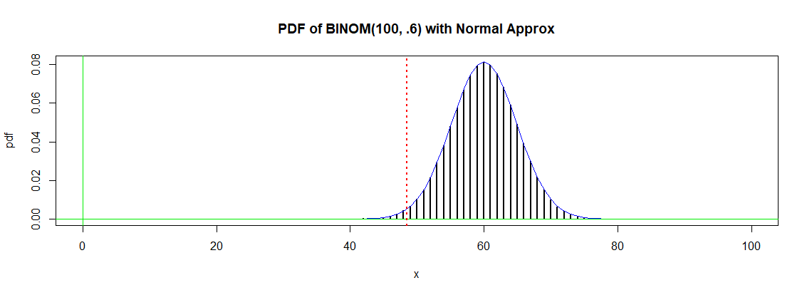
enter image description here

R code for graph:

x = 0:100;  p = .6
pdf = dbinom(x, 100, p)
hdr = "PDF of BINOM(100, .6) with Normal Approx" 
plot(x, pdf, type="h", lwd=2, main=hdr)
 curve(dnorm(x, 60, sqrt(24)), add=T, col="blue")
 abline(h=0, col="green2"); abline(v=0, col="green2")
 abline(v=48.5, col="red", lwd=2, lty="dotted")
$\endgroup$

Your Answer

By clicking “Post Your Answer”, you agree to our terms of service and acknowledge you have read our privacy policy.

Not the answer you're looking for? Browse other questions tagged or ask your own question.