Why do my Forecast vs Actual Graph using ARIMA look weird?

Question

I tried using ARIMA method to forecast yearly Wind speed data, using Diky fuller test P-value is below 0.05 hence I use the original data instead of differential. The data amounts 730, 2 sets of data for 1 day.

from statsmodels.tsa.arima_model import ARIMA

# 1,0,2 ARIMA Model
model = ARIMA(df, order=(1,0,2))
model_fit = model.fit(disp=0)
print(model_fit.summary())

This code gives me MA.L2.wind_speed: coeff= 0.1657, std error= 0.042, P>|z|=0

So I think I am good with this p, d and q value

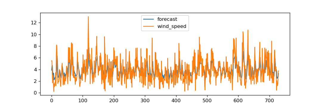
model_fit.plot_predict(dynamic=False)
plt.show()

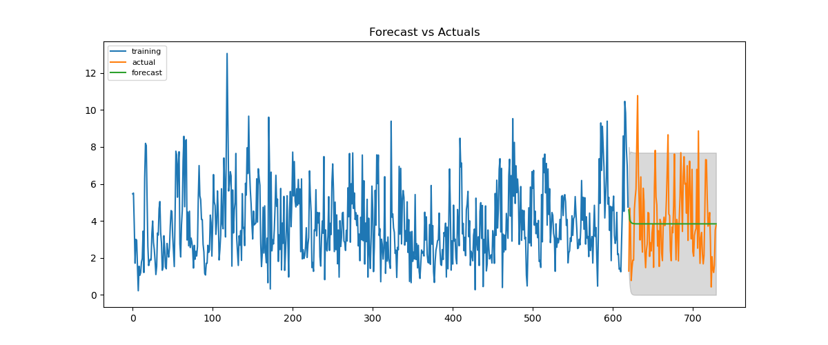
The actual vs fitting data does not look bad, but the issue comes from Out-of-time Validation graph

It looks too much different with the actual data. I use this code to for the forecast.

train = df[:620]


test = df[620:]

# Build Model
# model = ARIMA(train, order=(3,2,1))
model = ARIMA(train, order=(1, 0, 2))
fitted = model.fit(disp=-1)

# Forecast
fc, se, conf = fitted.forecast(110, alpha=0.05)  # 95% conf

# Make as pandas series
fc_series = pd.Series(fc, index=test.index)
lower_series = pd.Series(conf[:, 0], index=test.index)
upper_series = pd.Series(conf[:, 1], index=test.index)

What should I do to fix the forecast?

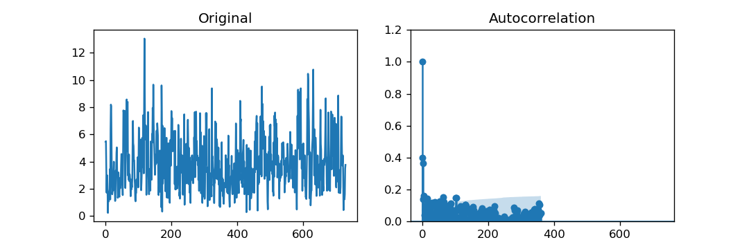
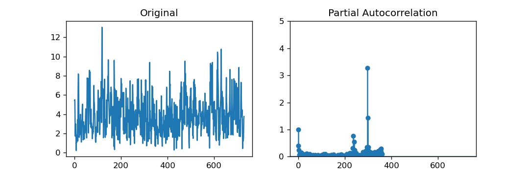
EDIT: Below is the picture of ACF and PCF I used to decide P and Q Value

P comes from Partial correlation that while I could not see the significance line, lag 1 has shown to be above it and safe enough to be used, CMIIW.

Q uses Auto correlation, I simply chose 2 because there are several lags above the line, so if 2 does not give good error I would change it into other numbers.

The Estimates from ARMA models are as follow: constant = 3.8709

ar.L1.wind_speed = 0.5320

ma.L1.wind_speed = -0.2129

ma.L2.wind_speed = 0.1657

Answer 1

It looks exactly as I would expect this kind of a model should forecast the mean.

This is an AR(1) model (ignoring MA terms here). It's of the form: $$x_t=c+\phi_1 x_{t-1}+\varepsilon_t$$

After a few steps its forecast becomes a straight line at $\bar\mu=\frac c {1-\phi_1}$ level. Even if you include MA terms the long run forecast is the same, only variance changes a bit. Information about the world at $I_{t-1}=x_{t-1}$ is lost at the rate of $(1-\phi_1)^h$ with $h$ being a period of forecast horizon. After a few steps none of the past matters except the long run mean $\bar\mu$

ARIMA models are great for short term forecasting, and also are useful to handle strong seasonality. They don't have a lot of structure, and are generally boring in long term forecasts without seasonality

Answer 2

I'll be hand-wavy but your outputs are fine for an ARIMA. The main difference between your two graphs of fitted and out of sample forecasts are that you are feeding actual past values in the top graph but your forecast uses past forecast values to forecast. Simple ARIMA orders will never have the bips and bops that your actual data has in it's forecast in a long forecast horizon. If there is some sense of seasonality or something you could:

1. De-seasonalize it and fit arima then add back in seasonality
2. Fit a SARIMAX which also comes with Statmodels
3. Fit some other model like a holt-winters or fbprophet

I personally recommend number 3!

And if there is no real seasonality then what the ARIMA has done is essentially cut through the noise and shown you the level of your inputs which is a reasonable thing to do.