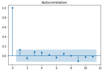
It seems to be a rule of thumb to use $\frac{1}{\sqrt n}$ as a standard error for an autocorrelation estimate of a time series, which then allows one to construct a confidence interval for sample autocorrelations which look something like this
I haven't encountered a derivation of this interval in econometrics textbooks and a quick google search does not yield immediate results. There has already been an attempt to address this questions on CV, see this post. Here are my thoughts, you feedback is welcome.
Attempt 1. Assume that the underlying observations are independent, i.e. $y_t$ are independent from each other with finite mean $\mu$ and variance $\sigma^2$. Then, autocorrelation of order $k$ is defined as $$r_k = \frac{Cov[y_t,y_{t-k}]}{\sigma^2}$$ and our estimator is $$ \begin{equation} \hat r_k = \frac{1}{\sigma^2}\frac{1}{T}\sum_{t=k+1}^T(y_t - \mu)(y_{t-k} - \mu), \tag{1} \end{equation} $$ where I assumed that $\sigma^2$ is known and not estimated to simplify things. By expanding the summation $$ \begin{align} \hat r_k &= \frac{1}{\sigma^2}\frac{1}{T}\sum_{t=k+1}^T(y_t - \mu)(y_{t-k} - \mu) \\ &= \frac{1}{\sigma^2}\left( \frac{1}{T}\sum_{t=k+1}^T y_ty_{t-k} - \mu\frac{1}{T}\sum_{t=k+1}^Ty_t - \mu\frac{1}{T}\sum_{t=k+1}^Ty_{t-k} + \mu^2 \right) \\ &= \frac{1}{\sigma^2} \left(\frac{1}{T}\sum_{t=k+1}^T y_ty_{t-k} - \mu^2 \tag{for big T}\right) \\ &\sim \frac{1}{\sigma^2} \frac{1}{\sqrt{T}} \times N\left( 0, \sigma^4 + 2\sigma^2\mu^2 \right) \tag{independence + CLT} \\ &= N\left( 0, \frac{1}{T} (1 + 2\frac{\mu^2}{\sigma^2}) \right). \end{align} $$ Setting $\mu=0$ (or less likely $\sigma=\infty)$ yields desired variance $T$, however this does not hold for $\mu \neq 0$. The independence assumption is stricter than $r_k=0$, however without it one could not apply a standard CLT. It could be relaxed to $y_t$ are martingale difference sequence and use appropriate CLT but his is still stronger than $r_k=0$.
Assuming only $r_k=0$ is what we ideally want but that would mean that $y_t$ is a white noise and I haven't found a CLT version that would apply then. Maybe you have other thoughts.
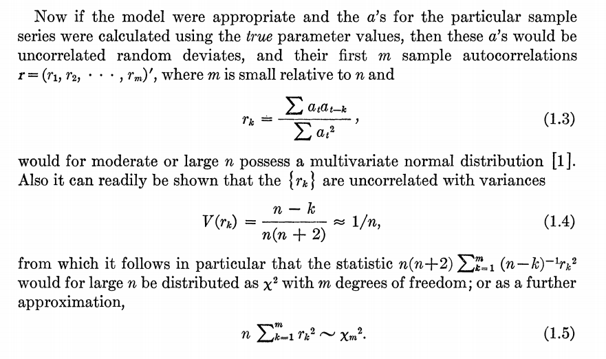
Attempt 2. There is a well known test for testing autocorrelation in residuals by Ljung and Box, see original paper. They apply it to ARIMA setting to test whether model residuals are autocorrelated. The main argument they use is the following
 where they make an underlying assumption that true errors $a_t$ are independent and normally distributed (they site this paper by Anderson for derivation). After that they state the variance for an autocorrelation of order $k$ is
$$
Var[r_k] = \frac{n-k}{n(n+2)} \approx \frac{1}{n}.
$$
My questions are:
- Do you have a derivation of the variance above?
- This is a finite sample variance (as opposed to asymptotic in Attempt 1) that is based on normality assumption which is hardly applicable in practice except maybe (auto)regression setting and testing model adequacy. Why is then standard to use it to test significance of autocorrelations estimated on time series data?
- Given the assumptions that are made, would it be correct to state that the null hypothesis of this test when applied to a time series data (not regression residuals) is $$ \begin{align} H_0&: y_t \quad \text{are i.i.d. normal} \\ H_A&: y_t \quad \text{are not i.i.d. normal} \end{align} $$ instead of $$ \begin{align} H_0&: \text{all autocorrelations are zero} \\ H_A&: \text{some autocorrelations are not zero} \end{align} $$ as usually stated when performing the test.
- Do you know any other ways to formally test whether empirical autocorrelations are different from zero?

