How do I have a p-value of 1 in the left tail from a two-sample t-test?

Question

I have a sample with a mean of 383.45, a standard deviation of 48.878, and a sample size of 30, and a second sample with a mean of 167.78, a standard deviation of 72.368, and a sample size of 30. When I perform a one-tailed two-sample t-test using a TI-84 Plus CE I get a t statistic of 13.52684957 and a p-value of 8.742353334e-19 for the right tail (μ1 > μ2) and 1 for the left (μ1 < μ2). As you might expect, My null hypothesis is that the populations for both samples have the same mean. My alternative hypothesis is that the first sample's population has a greater mean (μ1 > μ2). So, I plan on using the right tail but I'm confused as to why the left tail has a probability of 1 even though when I do a two-tailed test (μ1 ≠ μ2) I get a p-value of 1.748470667e-18 which is around double the p-value for the right tail.

Answer 1

The answer by @Dave2e is fine (+1), but I wanted to give an Answer based mainly on a specific example and showing computations of P-values.

Consider the following fictitious data:

set.seed(2022)
x1 = rnorm(30, 350, 50)
x2 = rnorm(30, 300, 70)

summary(x1);  length(x1);  sd(x1)
   Min. 1st Qu.  Median    Mean 3rd Qu.    Max. 
  205.0   309.6   346.7   344.2   379.2   410.6 
[1] 30         # sample size
[1] 46.29298   # sample SD

summary(x2);  length(x2);  sd(x2)
   Min. 1st Qu.  Median    Mean 3rd Qu.    Max. 
  190.9   281.3   310.5   307.6   353.5   418.5 
[1] 30
[1] 58.53848

Now, do a two sample Welch t test of $H_0: \mu_1=\mu_2$ against $H_a: \mu_1 > \mu_2,$ using t.test in R:

t.test(x1,x2, alt="gr")

        Welch Two Sample t-test

data:  x1 and x2
t = 2.6864, df = 55.074, p-value = 0.004764
alternative hypothesis: 
 true difference in means is greater than 0
95 percent confidence interval:
 13.8086     Inf
sample estimates:
mean of x mean of y 
 344.2034  307.5991 

The P-value of the test is computed by looking in the upper tail of Student's t distribution with 55.074 degrees of freedom. [DF is adjusted downward from $n_1+n_2-2=58$ to compensate for the difference in sample variances.]

1 - pt(2.6864, 55.074) 
[1] 0.004764504

[In R, pt is a CDF of Student's t distribution.]

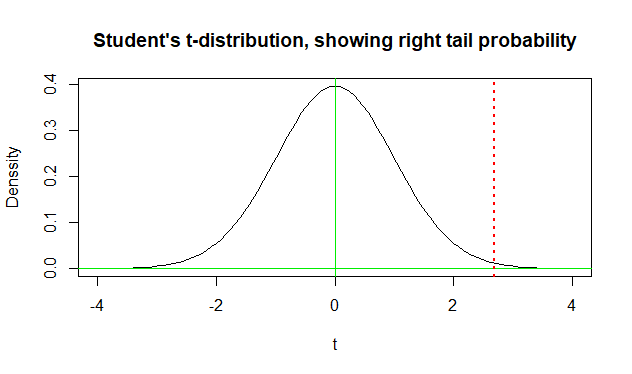
The P-value is the area under the density curve to the right of the vertical dotted red line.

R code for figure:

curve(dt(x, 55.074), -4, 4, 
         ylab="Denssity", xlab="t", main=hdr)
 abline(h=0, col="green2")
 abline(v=0, col="green2")
 abline(h= 2.6864, col="red", lwd=2, lty="dotted")
 abline(v= 2.6864, col="red", lwd=2, lty="dotted")

If you do a 2-sided t test, then the P-value is calculated by looking both in the lower tail below $-2.6864$ and in the upper tail above $2.6864.$ [By using $-notation, we show only the P-value.]

t.test(x1, x2)$p.val
[1] 0.009528523

This P-value for a 2-sided test is computed as follows:

pt(-2.6864, 55.074) + 1 - pt(2.6864, 55.074)  
   # left tail + right tail
[1] 0.009529008

Alternatively, using the symmetry of the t distribution:

2*pt(-2.6864, 55.074)   $ Double left tail probability 
[1] 0.009529008

Note: Quantities in the output of the test are rounded slightly to save space, so there is a tiny discrepancy with the P-values shown just above.

However, if you get confused (easy to do), and ask for the wrong side, using parameter alt="less" in t.test, then you get a nonsense P-value near $1.$

 t.test(x1, x2, alt="less")$p.val
 [1] 0.9952357

Answer 2

Let us define $\mu_1= 383$ and $\mu_2= 168$ with reasonable small standard deviations. The differences between the means are over 4 standard deviations apart. By eye one can judge, with a large difference, that it is very very unlikely to occur by chance alone.

With regard to a discussion of the formal analysis:

The right tail t-test is comparing if $\mu_1(383) > \mu_2(168)$ is clearly TRUE: thus a p-value of nearly 0.

The left tail t-test is testing whether $\mu_1(383) < \mu_2(168)$ which we can see is clearly FALSE: thus a very high p-value of nearly 1.

The null hypothesis $\mu_1(383) = \mu_2(168)$ we can also clearly see is thus FALSE given the relatively small standard deviations. Since we are allowing $\mu_1$ to be greater than or less than $\mu_2$ the probability is split on both sides of the normal distribution; thus the p-value is greater than for the right tail test.

Now if the means were closer or if the standard deviations were sufficiently large, the results would not be so clear cut and thus the recommendation to sketch out the distributions to verify the calculations makes sense.

Hope this answered your question.