Do you ever test the pre-asymptotic behaviour of a variable before performing a comparison of means t-test?

Question

I understand that it is not the normality of a random variable that matters in a t-test, but rather the fact that the distribution of the mean follows a normal distribution for large samples. However, is it sometimes useful to test how large a sample must be before the assumption of a normal distribution is warranted? For example, if the number of samples required were very large (much larger than n=30), would assuming a normal distribution be inappropriate? If so, how would you go about checking this?

The inspiration for this question comes from reading about Nassim Nicholas Taleb's Kappa metric.

Answer 1

Of course, the main issue is for the t statistic to have a t distribution with the appropriate degrees of freedom.

For normal data $\bar X$ and $S$ are stochastically independent. (One might argue that they are not functionally independent because $S^2$ can be defined in terms of $\bar X.)$ By contrast, for exponential data $\bar X$ and $S$ are not independent.

So, technically, it not enough for $n$ to be large enough that $\bar X$ is nearly normal. In order for the distribution of a t statistic, e.g, $T = \frac{\bar X-\mu_0}{S/\sqrt{n}},$ to have the appropriate t distribution, its numerator and denominator should be independent.

Using goodness-of-fit tests to check data for normality before doing a t test has been deprecated. But it is a good idea to look at plots of the data to see if they are nearly symmetrical and free of far outliers in either direction before using the data for a t test.

For example, consider a sample of size $n = 100$ from a Pareto distribution with minimum value $1$ and shape parameter $\alpha = 10,$ and mean $\mu = 10/9.$ [Observations can be sampled as $e^Y,$ where $Y\sim\mathsf{Exp}(\mathrm{rate}=10).]$ Each row of the matrix MAT below contains such a sample.

set.seed(2022)
m = 10^4;  n = 100
MAT = matrix(exp(rexp(m*n, 10)), nrow=m)

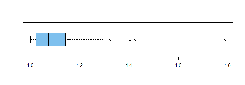
A boxplot of the first sample shows marked right-skewness and outliers.

boxplot(MAT[1,], horizontal=T, col="skyblue2")

a = rowMeans(MAT)
s = apply(MAT,1,sd)
cor(a, s)
[1] 0.7201542

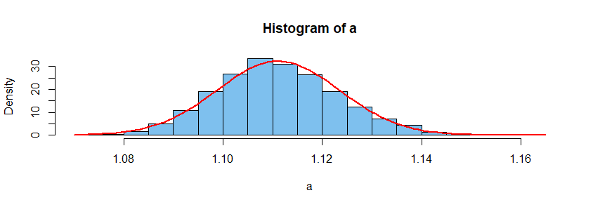
Sample means and SDs are clearly correlated. But one might consider that the means $\bar X$ (a in the code) are "close enough" to normal.

hist(a, prob=T, br=30, col="skyblue2")
 curve(dnorm(x,mean(a), sd(a)), add=T, col="red", lwd=2)

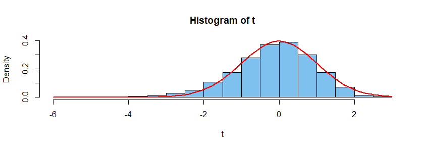
However, $T$ statistics are not distributed as $\mathsf{T}(\nu=99)$---especially not in the tails, where values are used to decide whether to reject the null hypothesis. So one should not trust results of a t test on such Pareto data.

t = (a - 10/9)/(s/sqrt(n))
hist(t, prob=T, br=30, col="skyblue2")
 curve(dt(x,n-1), add=T, lwd=2, col="red")

By contrast, samples of size $n = 50$ from a standard uniform distribution behave well.

set.seed(129)
m = 10^4;  n = 50
MAT = matrix(runif(m*n), nrow=m)
a = rowMeans(MAT);  s = apply(MAT,1,sd)
cor(a, s)
[1] -0.01452768   # nearly independent

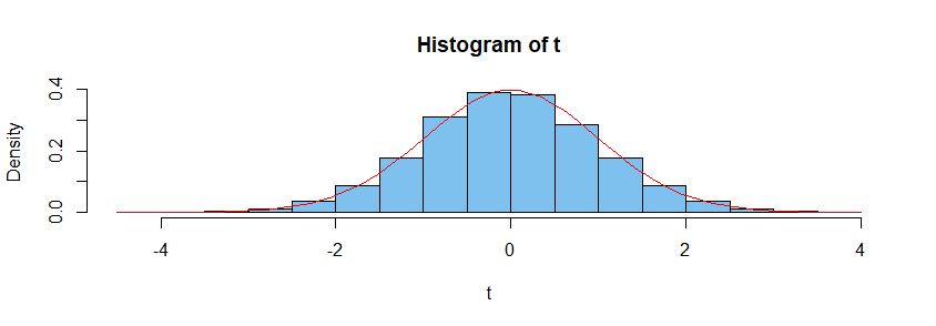
$T$ statistics are nearly distributed as $\mathsf{T}(\nu=49).$ So one could trust results of a t test on such uniform data.

t = (a - 1/2)/(s/sqrt(50))
hist(t, prob=T, br=20, col="skyblue2")
 curve(dt(x,49), add=T, col="red")

Answer 2

When you are using a statistical test that relies on the central limit theorem (as the T-test does), the test is only valid if the underlying distribution has a finite variance. If the underlying distribution of the data has sufficiently heavy tails that it does not have a finite variance then the central limit theorem does not apply and the test will not work properly. Thus, the most important preliminary issue for applying a T-test is whether or not the data come from a distribution where the rate of decay in the tails is sufficiently fast to give finite variance; anything faster than cubic decay is sufficient to give a finite variance.

To examine the rate of decay in the tails of a distribution, using a sample from that distribution, the usual diagnostic tool is a tail plot. You can find a related post here discussing the construction of a tail plot and the examination of the plot to see if the distribution has a finite variance. An example of tail plots for the two tails of a dataset is shown below.

Answer 3

I think the normality on the population does matter. It is a necessity for the t-distribution to hold. See my own question body for why.

So I think it is a good idea to check the normality of the population.

Note: when normality is not there, t-test has certain robustness against it, but that is another topic.