inferring heavy-tail distribution from finite sample of histogram data

Question

I have some data in the form of bins and counts. Here is one complete non-truncated example:

bins: 60-100, 100-200, 200-300, 300-500, 500-1000, 1000-2000, 2000-3000, >3000 
counts: 275, 320, 112, 65, 53, 44, 16, 15

Counts is the number of objects with sizes given by corresponding bin (60-100, 100-200 etc). If we construct the probability density function (dividing counts by bin size and scaling to total counts), we get some decreasing exp-like dependence. I have a hypothesis (and the nature of the objects implies so), that this may be the right-hand tail of a skewed Gaussian with its center somewhere out of measurements scope (for bins around 10 or less). But there is another idea, that this function may come from a long-tailed (or heavy-tailed) statistics.

(Update in clarification). Under "heavy-tailed" the stable distribution law is meant (in Levy sense) different from Gaussian, which in its intuitive concept involves: infinite dispersion or higher moments and asymptotics as x^-n instead of exp(-x^2).

Is it possible on the basis of these data only (I have several other such objects) to discriminate between exponential decrease and long-tail behaviour? Perhaps, with stating some confidence and probability of such hypothesis. What are tests which could answer this question and how they can be implemented preferably in R and/or in Mathematica? (other languages suit as well, if the solution exists therein).

In favour of this hypothesis is that the amount of matter for each bin (that is \int f(x)*x dx) increases with increased bin number, which seems to be not the case, if we had purely Gaussian tail.

If the sample is too sparse, and no conclusion can be drawn with reasonable confidence, how can I estimate the amount of needed data (number of bins and/or bin sizing) which are sufficient for this inference?

Answer 1

There are lots of ways to define "heavy tails" depending on which specific property is important, but a common definition is when the tails are heavy enough for the variance to be infinite. (This meaning is relevant in probability theory because it vitiates application of the central limit theorem.) In any case, it is possible to use the data to get an idea of the likely shape of the tails, though this always requires extrapolation beyond the data range.

---

Heavy-tailed distributions (infinite variance): Consider a density function $f$ with tails that decay according to the power-law:

$$f(x) \rightarrow c x^{-\omega-1} \quad \quad \text{as } x \rightarrow \infty.$$

From this form is it easy to show that:

$$\int \limits_x^\infty (r-\mu)^2 f(r) dr = \mathcal{O}(x^{2-\omega}),$$

so the upper-end of the integral converges to a finite value only if $\omega>2$. Hence, the variance of the distribution will be finite so long as both tails decay at least as fast as a power-law greater than cubic decay. It is important to note that heavy-tailed distributions only arise when the variable of interest is unbounded. If the variable of interest is bounded to some finite region then the variance must be finite and so no problem arises.

---

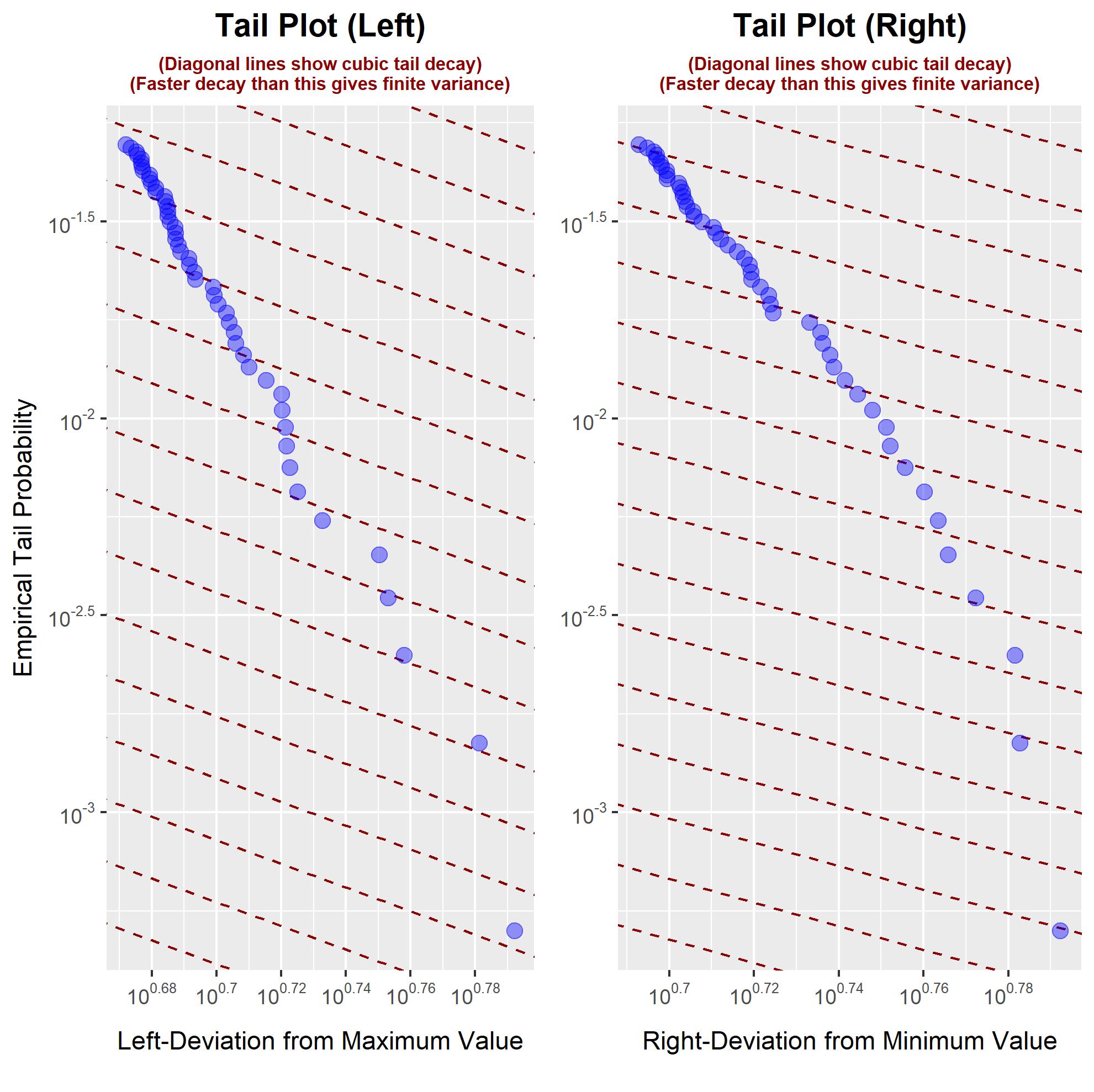
Looking at tail behaviour in the data: We can use the observed sample values in the tail of the distribution to see if this appears to be the case for our data. From the form of a density function with power-law decay, it is easy to show that the log-tail-probability and log-deviation from any fixed point $x_0$ are related in the tail by:

$$\ln \mathbb{P}(X>x) \rightarrow \text{const} - \omega \ln(x-x_0) \quad \quad \text{as } x \rightarrow \infty.$$

Letting $x_{(1)} \geqslant \cdots \geqslant x_{(n)}$ be the ordered sample values we can estimate the log-tail-probability by $\ln \hat{\mathbb{P}}(X>x_{(i)}) = \ln(2i-1)- \ln(2n)$. For the values occurring in the tails of the distribution we should therefore expect the values to follow the relationships:

$$\begin{matrix} \text{Right tail } & & & & \quad \quad \quad \ln(2i-1) \approx \text{const} - \omega \ln|x_{(i)}-x_0|, \\ \text{Left tail} \quad & & & & \text{ } \ln(2(n-i)-1) \approx \text{const} - \omega \ln|x_{(i)}-x_0|. \\ \end{matrix}$$

(Note that we are taking logarithms so we only look at the values on the appropriate side of the mean. This is reasonable since we are only interested in the tail values in each tail.) In order to diagnose whether there is evidence of heavy tails in the distribution we can construct tail plots which show the logarithmic terms in these approximate equations, and we can look at the slope of the relationship to estimate the value $\omega$ for each tail. The values in the tail-plots are given by:

$$\begin{matrix} \text{Vertical axis (Right tail) } & & & & \quad \quad \quad \ln(2i-1) \\ \text{Vertical axis (Left tail)} \quad & & & & \text{ } \ln(2(n-i)-1) \\ \text{Horizontal axis } \quad \quad \quad \quad & & & & \quad \quad \ln|x_{(i)}-x_0| \end{matrix}$$

Here is an example of this kind of plot for some data from a normal distribution. (This plot is produced using the tailplot function in the utilities package in R.) This plot shows log-deviations from the minimum/maximum sample values.

From these tail plots we see that both tails appear to be decaying faster than cubic decay. In interpreting these plots we concentrate on the values that are further into the tails, which are the values closer to the right-hand-side of each plot. It is important to note that a larger sample would show more values in the tails which might show a different rate of decay.

Answer 2

There are no agreed-upon definitions for long- and heavy-tailed. The power law definitions are often given, but they are too restrictive for practical purposes. The whole point of using such distributions is to model processes that produce occasional, extreme observations far in excess of what you would expect using the normal distribution. Such processes need not obey power laws or even have infinite support. For example, mix a U(-1,1) with a U(-10000, 10000), with mixing p=.0001 on the latter: This distribution has finite support, no power law, but is extremely heavy tailed. But using the power law definition, it is arguably "light-tailed."

Kurtosis measures (moment- and quantile-based) are useful alternative definitions of heavy-tailedness that do not have the limitations of the power law definitions.

Thus, as regards to the OP's data analysis question, I would suggest fitting the lognormal distribution using interval censored maximum likelihood, and then use the kurtosis of that fitted distribution as a measure of its heavy-tailedness. As far as the first category, you might question whether the interval is really 60-100 or 0-100. If 60 is really a hard-and-fast lower bound, then you need to modify the distribution. Otherwise, use 0-100 when fitting the lognormal.