Session using R:
(1) Nearly normal data: x1 no disease, x2 disease
summary(x1)
   Min. 1st Qu.  Median    Mean 3rd Qu.    Max.
  16.07   18.66   19.85   19.91   20.98   23.57
summary(x2)
   Min. 1st Qu.  Median    Mean 3rd Qu.    Max.
  19.90   22.39   23.09   23.36   24.52   27.34
Shapiro-Wilk tests may not be accurate for small samples.
Also, these data are rounded to two places and, strictly
speaking, rounded normal data are not exactly normal.
Nevertheless, both samples are consistent with samples
from normal populations, according to Shapio-Wilk tests:
shapiro.test(x1)$p.val
[1] 0.7933927
shapiro.test(x2)$p.val
[1] 0.9602677
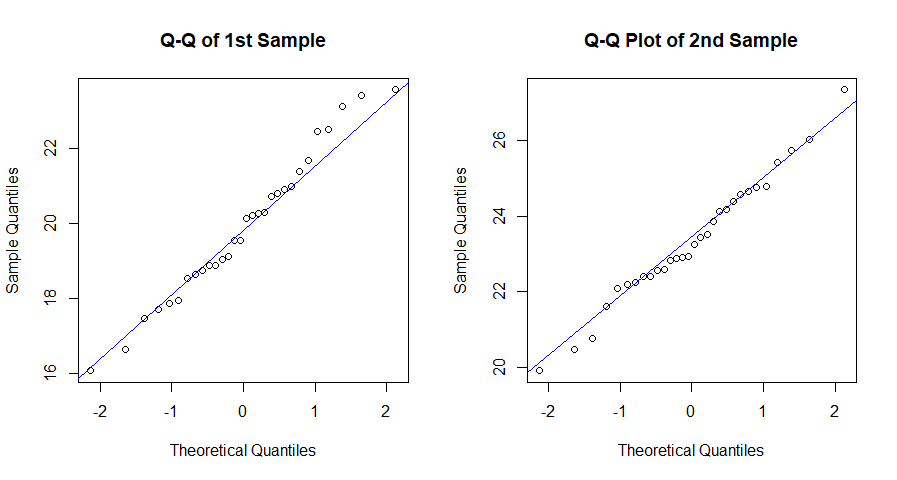
Many statisticians would prefer looking at normal Q-Q
plots to check for approximate normality. Plots should
be nearly linear (except possibly with some minor 'wobbles'
near the lower and upper tails). The plots below are
consistent with normal data.
par(mfrow=c(1,2))
 qqnorm(x1, main="Q-Q of 1st Sample")
  qqline(x1, col="blue")
 qqnorm(x2, main="Q-Q Plot of 2nd Sample")
  qqline(x2, col="blue")
par(mfrow=c(1,1))

A Welch 2-sample t test finds a significant difference
between the two sample means. (A Welch test does not
require equal variances and so is preferable to a pooled
test unless we have advance knowledge that populations
have equal variances)
t.test(x1, x2)

        Welch Two Sample t-test

data:  x1 and x2
t = -7.3334, df = 56.567, p-value = 9.217e-10
alternative hypothesis:
 true difference in means is not equal to 0
95 percent confidence interval:
 -4.393060 -2.508273
sample estimates:
mean of x mean of y
 19.90600  23.35667
(2) Right-skewed, non-normal data: y1 no disease, y2 disease
summary(y1)
   Min. 1st Qu.  Median    Mean 3rd Qu.    Max.
   5.29   13.16   16.77   19.61   24.30   43.87
 sd(y1)
 [1] 9.359215

summary(y2)
   Min. 1st Qu.  Median    Mean 3rd Qu.    Max.
   7.70   15.76   23.84   24.45   31.57   61.93
sd(y2)
[1] 11.37608
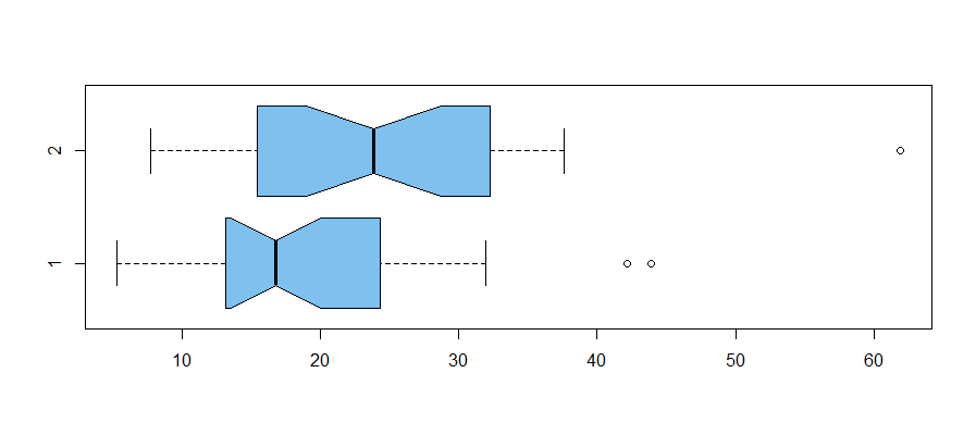
Boxplots (y1 bottom), show that both samples are moderately right-skewed with some boxplot outliers at the right. The 'notches' in
the sides of the boxes overlap, suggesting that we will
not find a significant difference in locations.
boxplot(y1,y2, col="skyblue2", horizontal=T,notch=T)

Neither sample passes the Shapiro-Wilk normality test; both
give P-values below 5%.
shapiro.test(y1)$p.val
[1] 0.04737606
shapiro.test(y2)$p.val
[1] 0.02658591
A 2-sample nonparametric Wilcoxon rank sum test does not find a significant difference in locations at the 5% level:
wilcox.test(y1, y2)

         Wilcoxon rank sum test

data:  y1 and y2
W = 329, p-value = 0.0747
alternative hypothesis:
 true location shift is not equal to 0
Note: You may find additional useful information
in some of the 'Related' links shown in the margin
of this page.


