I will try to answer this question based on what I understand from the article Bates et al. (2015), which is the same document as the lmer vignette cited in the question. The goal here is to better understand what the sum of squares for the fixed effect $i$ means, which is given by:
$$
\mathit{SS}_i = \hat{\beta}^\top \boldsymbol{R}_i^\top \boldsymbol{R}_i \hat{\beta}
$$
First of all, as it is stated in page 33 of the paper, $\boldsymbol{R}_i$ contain the rows of $\boldsymbol{R}_X$ associated with the $i$th fixed-effects term. The matrix $\boldsymbol{R}_X$ first appears in Eq. 18, on page 14. It is part of the Cholesky decomposition of the system matrix that appears in Eq. 17. This later matrix comes from the minimization of the penalized weighted residual sum-of-squares (Eq. 14), when the parameters $\boldsymbol{\theta}$ (the covariance parameter vector, associated with the random effects) are fixed.
Eq. 18 (and, also, Eq. 50) indicates how the matrix $\boldsymbol{R}_X$ is computed:
$$
\boldsymbol{R}_X^\top\boldsymbol{R}_X = \boldsymbol{X}^\top\boldsymbol{W}\boldsymbol{X} - \boldsymbol{R}_{ZX}^\top\boldsymbol{R}_{ZX}
$$
We will see later in this answer how this matrix $\boldsymbol{R}_X$ can be related to the sum of squares associated with the fixed effects. We will discuss later the meaning of the other two matrices ($\boldsymbol{X}$ and $\boldsymbol{R}_{ZX}$ that appear in the equation above.
Before getting to that, let us first consider a linear fixed-effects model, in which the response vector $\mathcal{Y}$ is normally distributed and whose mean value has a linear dependence on the fixed effects, represented by the $p$-dimensional coefficient vector $\boldsymbol{\beta}$:
$$
\mathcal{Y} \sim \mathcal{N}(\boldsymbol{X}\boldsymbol{\beta}, \sigma^2)
$$
Here, $\boldsymbol{X}$ is the $n\times p$ model matrix ($n$ is the number of observations, or the length of $\mathcal{Y}$). Note that this is similar to Eq. 1 of the paper, but I am considering $\boldsymbol{o}$ (the vector of known prior offset terms) to be equal to zero and $\boldsymbol{W}$ (the diagonal matrix of known prior weights) to be equal to the identity matrix, for sake of simplicity.
Let us make things concrete with an example in R. The code below prepares the data that will be used to fit both fixed-effects and mixed-effects models:
### number of levels of fixed effect x
p <- 2
### number of groups
q <- 4
### number of repetitions per level of x and per group
n <- 2
### Values for x
x <- rep(c(-1, 1), each = q * n)
### Groups
g <- gl(q, n, n * p * q)
### Fixed effects
fe.i <- 0.1
fe.x <- 0.5
### Random effects
set.seed(12345678)
re.i <- rnorm(q)
re.i <- 0.1 *(re.i - mean(re.i)) / sd(re.i)
re.x <- rnorm(q)
re.x <- 0.2 *(re.x - mean(re.x)) / sd(re.x)
### Noise
noise <- rnorm(n * p * q, sd = 0.3)
### Dependent variable
y <- fe.i + fe.x * x + re.i [g] + re.x [g] * x + noise
### Data frame
dat <- data.frame(x = x, y = y, g = g)
Note that the factor x is continuous and was chosen such that there is no interaction between the fixed effects intercept and slope.
The fixed-effects linear model described above is fitted, in R, as follows:
m1 <- lm(y ~ x, dat)
The fitted coefficients $\hat{\boldsymbol{\beta}}$ can be extracted as:
m1.beta <- coefficients(m1)
whose values are:
> m1.beta
(Intercept)           x
  0.1492887   0.4151967
The model matrix $\boldsymbol{X}$ can be composed as:
X.m1 <- cbind(rep(1, n * p * q), x)
Assuming that:
$$
\boldsymbol{y}_{\mathrm{obs}} = \boldsymbol{X}\hat{\boldsymbol{\beta}} + \boldsymbol{\varepsilon}
$$
where $\boldsymbol{\varepsilon}$ is the vector of residuals with mean equal to zero and standard deviation $\sigma$, the total sum of squares $\mathit{SS}_\mathrm{total}$ can be related to the sum of squares due to the fixed coefficients $\mathit{SS}_\mathrm{fixef}$ and to the sum squares of the residuals $\mathit{SS}_\mathrm{resid}$:
$$
\mathit{SS}_\mathrm{total} = \mathit{SS}_\mathrm{fixef} + \mathit{SS}_\mathrm{resid}
$$
where:
$$
\begin{align}
\mathit{SS}_\mathrm{total} &= \boldsymbol{y}_{\mathrm{obs}}^\top\boldsymbol{y}_{\mathrm{obs}}\\
\mathit{SS}_\mathrm{fixef} &= \hat{\boldsymbol{\beta}}^\top\boldsymbol{X}^\top\boldsymbol{X}\hat{\boldsymbol{\beta}}\\
\mathit{SS}_\mathrm{resid} &= \boldsymbol{\varepsilon}^\top\boldsymbol{\varepsilon}
\end{align}
$$
These values can be computed as follows:
SS.fixef <- t(m1.beta) %*% t(X.m1) %*% X.m1 * m1.beta
SS.m1.resid <- sum(residuals(m1) ^ 2)
and are visualized with the following code:
> cat(sprintf("SS.fixef: %f (intercept), %f (slope)\nSS.resid: %f\n",
+            SS.fixef[1], SS.fixef[2], SS.m1.resid))
SS.fixef: 0.356594 (intercept), 2.758212 (slope)
SS.resid: 2.141890
Note that, when computing SS.fixef, the last multiplication is scalar (*) instead of matrix (%*%), such that the sums of squares for both intercept and slope are computed separately.
The total sum of squares is computed as follows:
SS.total <- t(dat$y) %*% dat$y
and we can verify that the equation $\mathit{SS}_\mathrm{total} = \mathit{SS}_\mathrm{fixef} + \mathit{SS}_\mathrm{resid}$ holds:
> cat(sprintf("SS.total: %f\nSS.fixef + SS.resid: %f\n",
+             SS.total, sum(SS.fixef) + SS.resid))
SS.total: 5.256697
SS.fixef + SS.m1.resid: 5.256697
The values for the sums of squares for the slope (dependent on variable x) and for the residuals, which are respectively 2.75821 and 2.1419, are the identical to the ones that are obtained by the call of the anova function on model m1:
> anova(m1)
Analysis of Variance Table

Response: y
          Df Sum Sq Mean Sq F value    Pr(>F)
x          1 2.7582 2.75821  18.029 0.0008145 ***
Residuals 14 2.1419 0.15299
---
Signif. codes:  0 ‘***’ 0.001 ‘**’ 0.01 ‘*’ 0.05 ‘.’ 0.1 ‘ ’ 1
Let us now investigate the mixed-effects model and how it deals with the same data. According to Bates al. (2015), the conditional distribution of $\mathcal{Y}$ given $\mathcal{B} = \boldsymbol{b}$ has the form:
$$
(\mathcal{Y}|\mathcal{B} = \boldsymbol{b}) \sim \mathcal{N}(\boldsymbol{X}\boldsymbol{\beta} + \boldsymbol{Z}\boldsymbol{b}, \sigma^2)
$$
where $\boldsymbol{Z}$ is the $n \times q$ model matrix for the $q$-dimensional vector-valued random-effects variable, $\mathcal{B}$, whose value is fixed at $\boldsymbol{b}$. The unconditional distribution of $\mathcal{B}$ is also multivariate normal with mean zero and a $q \times q$ variance-covariance matrix $\boldsymbol{\Sigma}$. Again, the matrix of weights $\boldsymbol{W}$ is ignored here for the sake of simplicity.
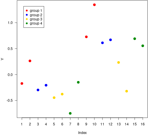
Note that in the data defined above (included in the data frame dat), there is a grouping factor g, which has four levels. For each one of these levels, there are two measurements for $x = -1$ and another two measurements for $x = 1$. The data has been generated such that random effects on both intercept (with size re.i) and slope (with size re.x) are induced. With 16 observations in total, it is possible to fit a model containing random effects for both intercept and slope, avoiding singularities in the fit.
This is a graphical representation of the data:
png(file = "data.png", width = 500, height = 470)
par(mar = c (5, 4, 0.1, 0.1))
cols <- c("red", "blue", "gold", "green4")
plot(dat$y, las = 1, pch = 19, col = cols[dat$g],
     ylab = "Y", cex = 1.5, xaxt = "n")
axis(1, at = seq (1, nrow (dat)))
legend("topleft", ins = 0.05, col = cols, pch = 19,
       legend = sapply (seq (1, q), function (x) sprintf ("group %d", x)))
dummy <- dev.off()

The horizontal axis is just the row index of data frame dat. The value of $x$ for the first 8 points is $-1$ and the value of $x$ for the last 8 points is $1$.
We fit a mixed-effects model with two fixed factors (for intercept and slope) and with two random factors, specified by the formula element (x || g), which is equivalent to (1 | g) + (0 + x | g) (i.e., we do not consider a correlation between random effects for intercept and slope):
library(lme4)
m2 <- lmer(y ~ x + (x || g), dat)
The fitted fixed coefficients $\hat{\boldsymbol{\beta}}$ can be extracted from the m2 object with this code:
m2.beta <- fixef(m2)
They are identical to the coefficients fitted to the fixed-effects model m1:
> cat(sprintf("FE model: intercept = %f, slope = %f\nME model: intercept = %f, slope = %f\n",
+            m1.beta[1], m1.beta[2], m2.beta[1], m2.beta[2]))
FE model: intercept = 0.149289, slope = 0.415197
ME model: intercept = 0.149289, slope = 0.415197
The model matrix $\boldsymbol{X}$ for m2 can be extracted with the following code:
X.m2 <- getME(m2, "X")
XtX <- t(X.m2) %*% X.m2
It is identical to the model matrix for m1:
> X.m1
         x
 [1,] 1 -1
 [2,] 1 -1
 [3,] 1 -1
 [4,] 1 -1
 [5,] 1 -1
 [6,] 1 -1
 [7,] 1 -1
 [8,] 1 -1
 [9,] 1  1
[10,] 1  1
[11,] 1  1
[12,] 1  1
[13,] 1  1
[14,] 1  1
[15,] 1  1
[16,] 1  1
> X.m2
   (Intercept)  x
1            1 -1
2            1 -1
3            1 -1
4            1 -1
5            1 -1
6            1 -1
7            1 -1
8            1 -1
9            1  1
10           1  1
11           1  1
12           1  1
13           1  1
14           1  1
15           1  1
16           1  1
attr(,"assign")
[1] 0 1
attr(,"msgScaleX")
character(0)
We can easily see that the values of $\hat{\boldsymbol{\beta}}^\top\boldsymbol{X}^\top\boldsymbol{X}\hat{\boldsymbol{\beta}}$
are the same for m1 and m2:
> t(m1.beta) %*% t(X.m1) %*% X.m1 %*% m1.beta
         [,1]
[1,] 3.114806
> t(m2.beta) %*% XtX %*% m2.beta
         [,1]
[1,] 3.114806
Remember that this was the value for the sum of squares associated with the fixed factors in the fixed-effects models. This is not the case for the mixed-effects model and we reach now the important point of this answer. As we have seen at the beginning of my text, $\boldsymbol{X}^\top\boldsymbol{X}$ is the sum of two terms (ignoring the $\boldsymbol{W}$ matrix, for the sake of simplicity):
$$
\boldsymbol{X}^\top\boldsymbol{X} = \boldsymbol{R}_X^\top\boldsymbol{R}_X + \boldsymbol{R}_{ZX}^\top\boldsymbol{R}_{ZX}
$$
Pre-multiplying by $\hat{\boldsymbol{\beta}}^\top$ and post-multiplying by $\hat{\boldsymbol{\beta}}$ both sides of the equation above:
$$
\hat{\boldsymbol{\beta}}^\top\boldsymbol{X}^\top\boldsymbol{X}\hat{\boldsymbol{\beta}} = \hat{\boldsymbol{\beta}}^\top\boldsymbol{R}_X^\top\boldsymbol{R}_X\hat{\boldsymbol{\beta}} + \hat{\boldsymbol{\beta}}^\top\boldsymbol{R}_{ZX}^\top\boldsymbol{R}_{ZX}\hat{\boldsymbol{\beta}}
$$
gives us an expression for the sums of squares that are related to fixed coefficients of the model. The right-hand side is the sum of squares of the fixed-effects model fitted to the same data. We see that this value is partitioned into two terms:
- the term $\hat{\boldsymbol{\beta}}^\top\boldsymbol{R}_X^\top\boldsymbol{R}_X\hat{\boldsymbol{\beta}}$ that is related to the fixed-effects coefficients per se,
- and the term $\hat{\boldsymbol{\beta}}^\top\boldsymbol{R}_{ZX}^\top\boldsymbol{R}_{ZX}\hat{\boldsymbol{\beta}}$ that appears because we are fitting a mixed-effects linear model to the data. Its value depends on the model matrix for the random effects $\boldsymbol{Z}$ and on the values of the parameters $\boldsymbol{\theta}$ of the variance-covariance matrix $\boldsymbol{\Sigma}_\boldsymbol{\theta}$. It is computed during the algebraic phase of the penalized least squares algorithm (Eq. 49).
This is why one should only consider the term $\hat{\boldsymbol{\beta}}^\top\boldsymbol{R}_X^\top\boldsymbol{R}_X\hat{\boldsymbol{\beta}}$ when computing the $F$ statistics for testing the fixed effects. One further indication that this must the case comes from the fact that the covariance matrix of the fixed-effects coefficients is given by (Eq. 54 of Bates et al. 2015):
$$
\mathrm{Var}_{\boldsymbol{\theta}, \sigma}(\hat{\boldsymbol{\beta}}) = \sigma^2 \boldsymbol{R}_X^{-1} (\boldsymbol{R}_X^\top)^{-1}
$$
and depends only on $\boldsymbol{R}_X$, besides $\sigma$.
The total sum of squares for the mixed-effects model can then be partitioned into four terms:
$$
\mathit{SS}_\mathrm{total} = \mathit{SS}_{RX} + \mathit{SS}_{RZX} + \mathit{SS}_\mathrm{ranef} + \mathit{SS}_\mathrm{resid}
$$
where:
$$
\begin{align}
\mathit{SS}_{RX} &= \hat{\boldsymbol{\beta}}^\top\boldsymbol{R}_X^\top\boldsymbol{R}_X\hat{\boldsymbol{\beta}}\\
\mathit{SS}_{RZX} &= \hat{\boldsymbol{\beta}}^\top\boldsymbol{R}_{ZX}^\top\boldsymbol{R}_{ZX}\hat{\boldsymbol{\beta}}\\
\end{align}
$$
The term $\mathit{SS}_\mathrm{resid}$ is only related to the residuals error (the value of $\sigma$) and the term $\mathit{SS}_\mathrm{ranef}$ is only related to the random effects (the values in the variance-covariance matrix of the random effects $\boldsymbol{\Sigma}_\boldsymbol{\theta}$).
In our example, this is how these values are computed:
RX <- getME(m2, "RX")
RZX <- getME(m2, "RZX")
RXtRX <- t(RX) %*% RX
RZXtRZX <- t(RZX) %*% RZX
SS.RX <- t(m2.beta) %*% RXtRX * m2.beta
SS.RZX <- t(m2.beta) %*% RZXtRZX %*% m2.beta
SS.m2.resid <- sum((dat$y - predict(m2)) ^ 2)
SS.ranef <- sum((dat$y - predict(m2, re.form=NA)) ^ 2) - SS.m2.resid
As we did previously, the last multiplication in the computation of SS.RX is scalar (*) instead of matrix (%*%), such that we can get the separated sums of squares for the intercept and the slope (this is another way of computing $\mathit{SS}_i$ with $\boldsymbol{R}_i$, as stated at the beginning of this answer).
We can verify that all terms sum up to the value of the total sum of squares ($\mathit{SS}_{\mathrm{total}}$):
> cat(sprintf("SS.RX: intercept = %f, slope = %f\nSS.RZ: %f\nSS.ranef: %f\nSS.m2.resid: %f\n\nSS.RX + SS.RZ + SS.ranef + SS.m2.resid: %f\nSS.total: %f\n",
+             SS.RX[1], SS.RX[2], SS.RZX, SS.ranef, SS.m2.resid,
+             sum(SS.RX) + SS.RZX + SS.ranef + SS.m2.resid,
+             SS.total))
SS.RX: intercept = 0.070573, slope = 2.181704
SS.RZ: 0.862529
SS.ranef: 1.270335
SS.m2.resid: 0.871556

SS.RX + SS.RZ + SS.ranef + SS.m2.resid: 5.256697
SS.total: 5.256697
As it should be, the value for the sum of squares for the fixed-effect slope (SS.RX[2]) is exactly the same as the value that appears when anova is invoked for m2:
> anova(m2)
Analysis of Variance Table
  npar Sum Sq Mean Sq F value
x    1 2.1817  2.1817  27.452
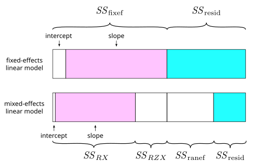
So to summarize, the value of the sum of squares associated with the coefficients of a mixed-effects model is somehow related to the sum of squares associated with the coefficients of the equivalent fixed-effects model fitted to the same data, in the sense that the former is a part of the later. This can be visualized in the figure below, where the width of the rectangles are proportional to the respective sums of squares (see Appendix for the code that generates part of this figure).

In this figure, the pink and the cyan rectangles correspond to the sums of squares that are used to compute the $F$ statistics that appear in the ANOVA tables, for both fixed-effects and mixed-effects models.
References
Bates D, Mächler M, Bolker B, Walker S (2015) Fitting linear mixed-effects models using lme4. J Stat Softw 67(1). DOI: 10.18637/jss.v067.i01.
Appendix
This is the code for generating part of the last figure. The generated SVG file was further edited in Inkscape for adding the labels.
svg(file = "ss.svg", width = 7, height = 4)
plot(NA, NA, type = "n", bty = "n", xaxt = "n", yaxt = "n",
     xlab = "", ylab = "", xlim = c(0, SS.total), ylim = c(0, 2.5))
y <- c(0, 0, 1, 1, 0)
x <- c(0, 1, 1, 0, 0)
o <- 0
for (s in c (SS.fixef[1], SS.fixef[2], SS.m1.resid)) {
    polygon(o + x * s, y + 1.5)
    o <- o + s
}
o <- 0
for (s in c (SS.RX[1], SS.RX[2], SS.RZX, SS.ranef, SS.m2.resid)) {
    polygon(o + x * s, y)
    o <- o + s
}
dummy <- dev.off()


