I need to build an overall survival regression model that can show the survival plots for id's with multiple rows.
I have used the Weibull function to define the baseline hazard function h0(t) and Cox hazard model to evaluate the effect of covariates.
Then I evaluated the hazard function h(t), followed by cumulative hazard function H(t), and finally the survival function S(t).
Can somebody please let me know if the steps that I have followed is correct or not in Python?
Here is what I have done:
Step-1: Import libraries
#Load the required libraries
import pandas as pd
pd.set_option('display.max_rows', 50)
pd.set_option('display.max_columns', 10)
pd.set_option('display.width', 1000)
import numpy as np
import matplotlib.pyplot as plt
from lifelines import WeibullFitter, CoxTimeVaryingFitter
from scipy import integrate
Step-2: Create dataset
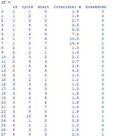
The dataframe has 4 id's/machines each having multiple rows and columns as 'cycle', 'start','Covariate', and 'breakdown'.
id-1 has 8 cycles.
id-2 has 6 cycles.
id-3 has 10 cycles.
id-4 has 4 cycles.
At the end of each cycle the event/breakdown of that specific id/machine is 1
data = {'id': [1, 1, 1, 1, 1, 1, 1, 1,
           2, 2, 2, 2, 2, 2,
           3, 3, 3, 3, 3, 3, 3, 3, 3, 3,
           4, 4, 4, 4],
    'cycle': [1, 2, 3, 4, 5, 6, 7, 8,
              1, 2, 3, 4, 5, 6,
              1, 2, 3, 4, 5, 6, 7, 8, 9, 10,
              1,2,3,4],
    'start': [0, 1, 2, 3, 4, 5, 6, 7,
              0, 1, 2, 3, 4, 5,
              0, 1, 2, 3, 4, 5, 6, 7, 8, 9,
              0, 1, 2, 3],
    'Covariate: x': [1.4,  1.9,  2.7,  3.8,  5.3,  7.4,  10.3,  14.4,
                  1.3,  1.6,  2.1,  2.7,  3.5,  4.2,
                  1.0,  1.1,  1.2,  1.3,  1.4,  1.5,   1.6,   1.8,  1.9,  2.1,
                  0.5,  1.0,  1.5,  2.0],
    'breakdown': [0, 0 ,0, 0, 0, 0, 0, 1,
                  0, 0, 0, 0, 0, 1,
                  0, 0, 0, 0, 0, 0, 0, 0, 0, 1,
                  0, 0, 0, 1],
    }


#Convert to dataframe
df = pd.DataFrame(data)
print("df = \n", df)
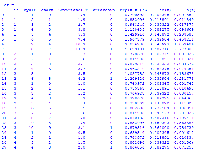
The above dataframe looks as such:
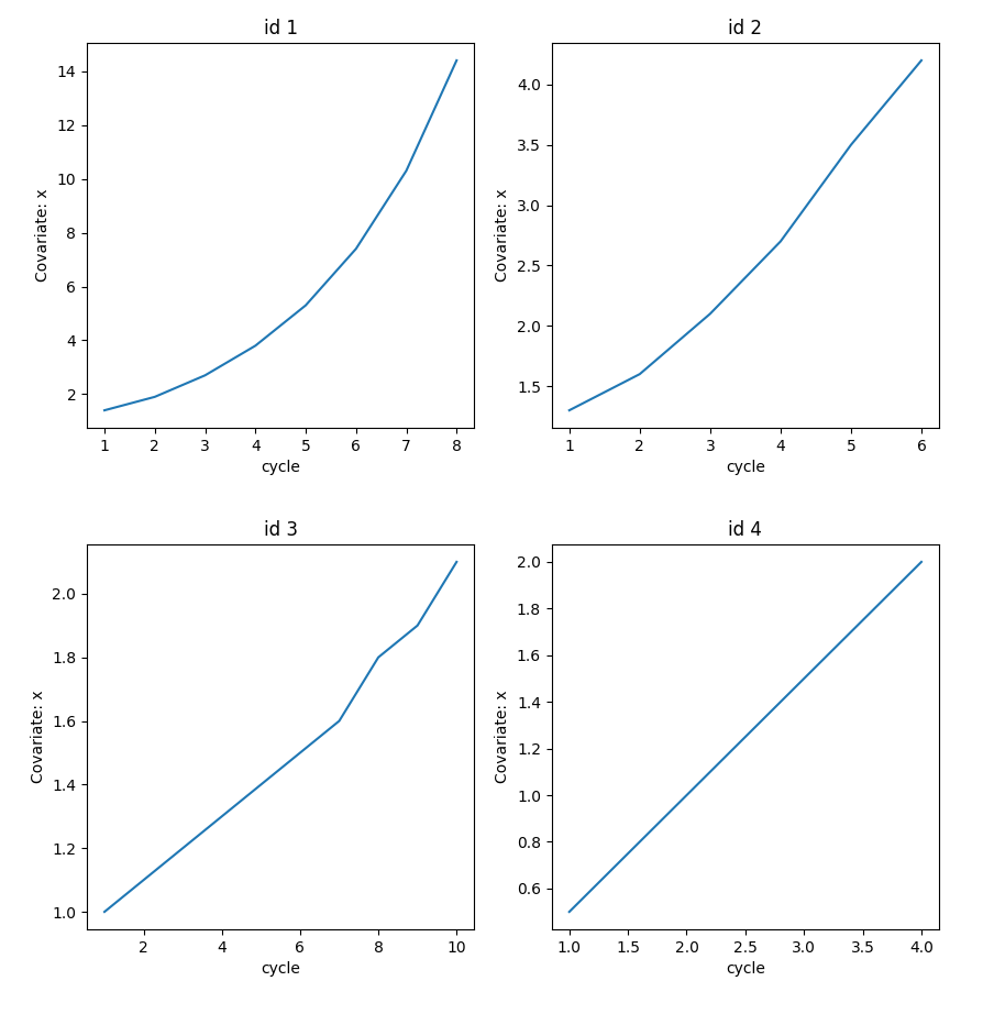
Here, the plot of cycle vs covariate/feature for each id/machine until breakdown is as shows:
Step-3: Instantiate CoxTimeVaryingFitter() to calculate partial hazard ratios: HR = exp(x−x¯)'β
The partial hazard ratios is represented as:
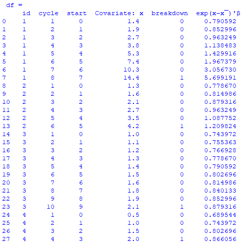
The value of "exp(x−x¯)'β" is evaluated as such:
## Instantiate the Cox Time Varying Fitter
## Reference: https://lifelines.readthedocs.io/en/latest/fitters/regression/CoxTimeVaryingFitter.html
ctv = CoxTimeVaryingFitter(penalizer=0)


## Fit the Cox Time Varying Fitter model
ctv.fit(df,
        id_col="id",
        event_col='breakdown',
        start_col='start',
        stop_col='cycle',
        show_progress=True)


## Print the summary of the model
ctv.print_summary()


## Plot the Regression coeff β
fig_verify = plt.figure(figsize=(15,7))
ctv.plot()
plt.title("Regression coeff β")
plt.show()


## Evalauate the partial hazard ratios: HR = exp(x−x¯)'β
df_LogPartialHazard = ctv.predict_partial_hazard(df)


## Append the partial hazard ratios (HR) to the dataframe
df['exp(x−x¯)′β'] = df_LogPartialHazard
The dataframe now looks as such:
Step-4: Instantiate WeibullFitter() to calculate the scale (λ) and shape parameters (ρ)
Here, we assume that the baseline hazard function for all the rows of a particular id is same.
The baseline hazard function is represented as:
The scale (λ) and shape parameters (ρ) are evaluated by considering the last row of every id when the machine breakdown by Instantiating the WeibullFitter().
## Get the last value of ['cycle','breakdown'] for every 'id'
weibull_data = pd.DataFrame(df.groupby('id')[['cycle','breakdown']].max()).reset_index()
The above data for WeibullFitter() looks as such:
## Instantiate WeibullFitter class
## Reference: https://lifelines.readthedocs.io/en/latest/fitters/univariate/WeibullFitter.html
wbf = WeibullFitter()


##Fit the WeibullFitter to data
wbf.fit(weibull_data['cycle'], weibull_data['breakdown'])


## WeibullFitter summary
print("\n wbf.summary = \n",wbf.summary)


## WeibullFitter model parameters
print("\n Scale parameter = λ_wbf = ",wbf.lambda_)
print("\n Shape parameter = ρ_wbf = ",wbf.rho_)


## AIC of Weibull model
print ("\n Akaike information criterion = ", wbf.AIC_)


## Loglikelihood for weibull dist
wei = wbf.log_likelihood_
print("\n Loglikelihood = ", round(wei,2))
The shape and scale parameters are evaluated as:
Step-5: Create baseline hazard function [ho(t)] for all the rows in the dataset using the scale (λ) and shape parameters (ρ)
## Create baseline hazard function [ho(t)] for all the rows in the dataset
def baseline_hazard(t,ρ,λ):
    h_0 = (ρ/λ) * ((t/λ)**(ρ-1))
    return h_0

## Baseline hazard function
df['ho(t)'] = baseline_hazard(t = df['cycle'] ,ρ = wbf.rho_, λ = wbf.lambda_)
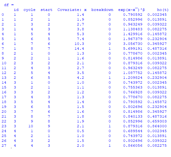
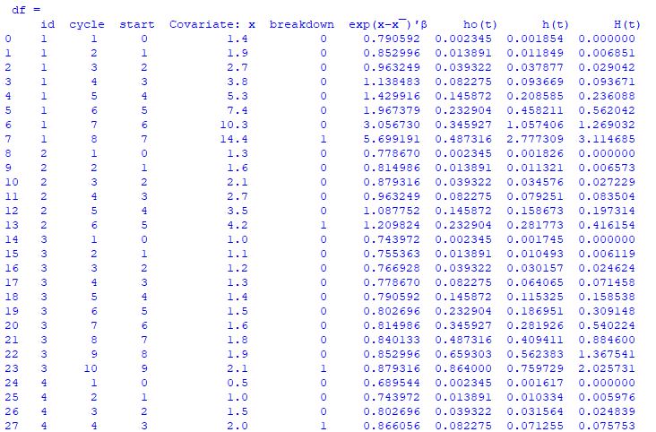
The dataframe looks as such:
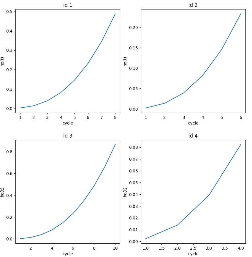
The baseline hazard function 'ho(t)' for all the id's looks as such:
Step-6: Create hazard function [h(t)] for all the rows in the dataset
The hazard function is given as such
## Hazard function: h(t) = ho(t)* exp(Xβ)
df['h(t)'] = df['exp(x−x¯)′β'] * df['ho(t)']
print("\n df = \n",df)
The dataframe looks as such:
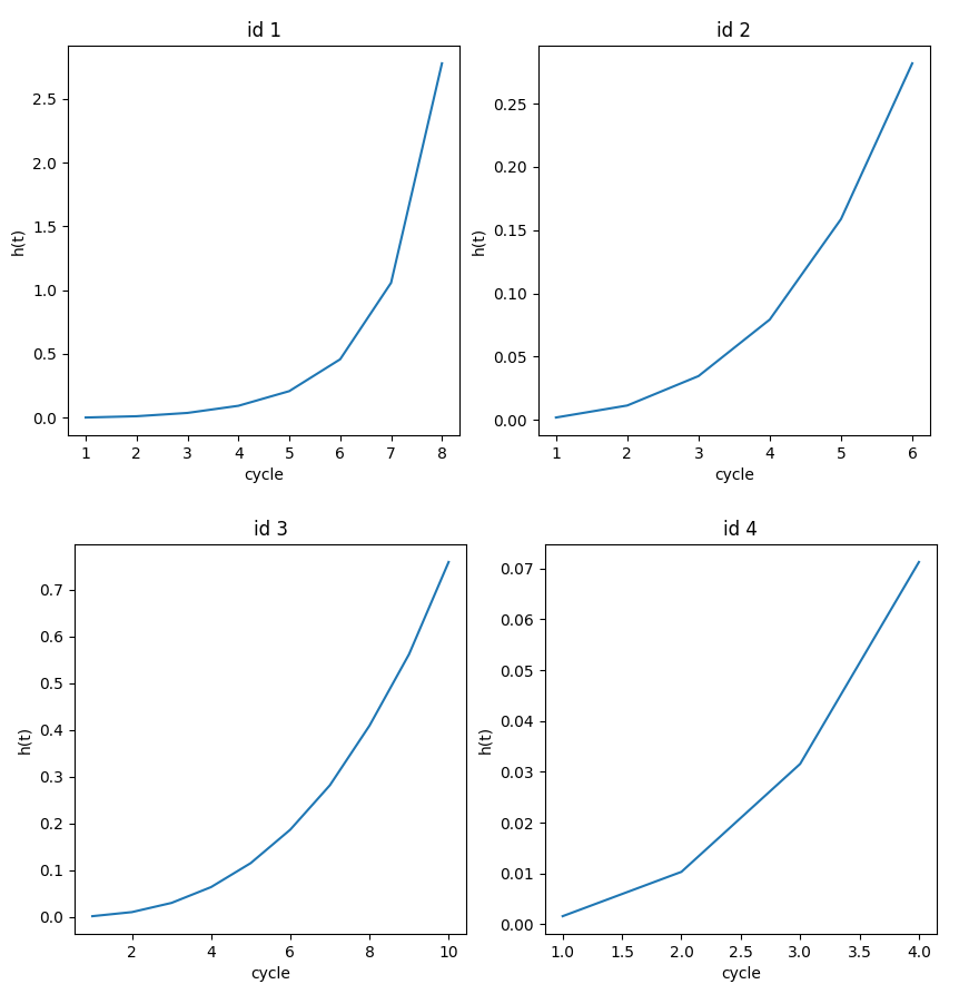
The hazard function 'h(t)' for all the id's looks as such:
Step-7: Calculate the cumulative hazard function H(t)
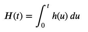
The cumulative hazard function H(t) is represented as:
Here we apply the simpson integration rule to evaluate the H(t) for every id
## Create function to evaluate cumulative hazard finction H(t)
def CUMULATIVE_HAZARD(complete_dataframe):

    ## Get the total number of cycles for each id
    grouped_by_unit = complete_dataframe.groupby(by="id")

    ## Create empty array for all the unique number of id's
    Cum_Haz_func_id = np.empty((np.int64(np.shape(complete_dataframe['id'].unique())[0]),0))

    ## Iterate over unique umber of id's
    for j in range (0,len(complete_dataframe['id'].unique())) :

        ## Rows of a particular id
        df_each_id = grouped_by_unit.get_group(j+1).reset_index()

        ## Empty array for rows of a particular id
        Cum_Haz_func_j_id = np.empty((np.int64(np.shape(df_each_id.index)[0]),0))

        ## Iterate over all the rows in a particular id
        for i in range (0,len(df_each_id.index)) :
            x = df_each_id['h(t)'][0:df_each_id.index[i]+1].reset_index()
            X = x['index']
            Y = x['h(t)']

            ## Integration via simpson rule
            Cum_Haz_func_in_j_ID_i_DataPoint = integrate.simps(Y, X)

            ## Append for the rows of a specific id
            Cum_Haz_func_j_id = np.append( Cum_Haz_func_j_id, Cum_Haz_func_in_j_ID_i_DataPoint)

        ## Append for all the rows for all the id's
        Cum_Haz_func_id = np.append( Cum_Haz_func_id, Cum_Haz_func_j_id)

    return Cum_Haz_func_id


## Cumulative Hazard function
df['H(t)'] = CUMULATIVE_HAZARD(df)
The dataframe looks as such:
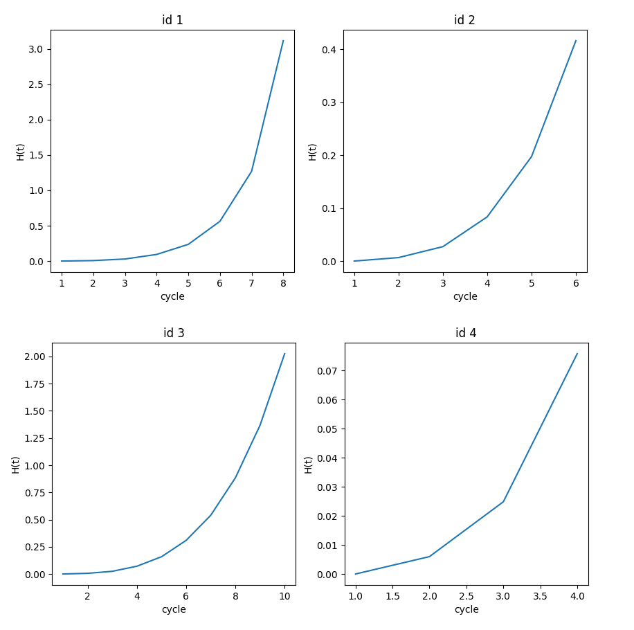
And the Cumulative Hazard function 'H(t)' for each id looks as such:
Step-8: Calculate the survival function S(t)
The survival function is written as:
## Survival function
df['S(t)'] = np.exp(-df['H(t)'])
print(" \n df = \n", df)
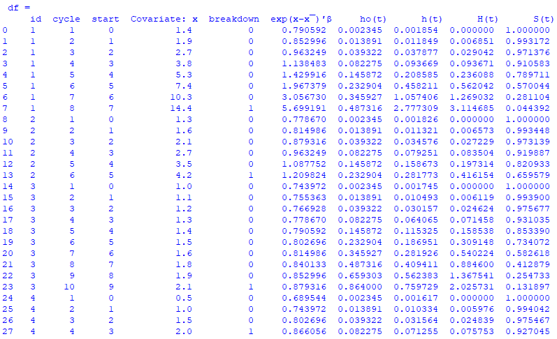
The above dataframe looks as such:
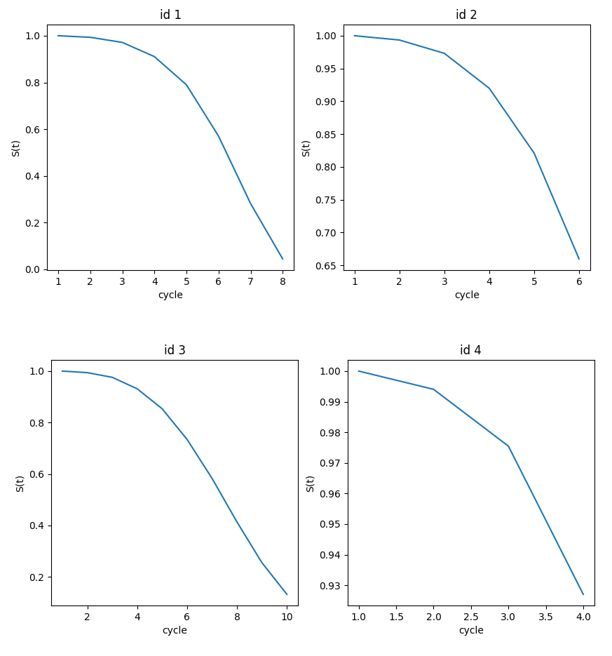
The survival function of each id looks as:
Now, can somebody please let me know if the above process to obtain the survival function plot for each id is correct or not?
Edit-1
The cumulative baseline hazard can be extracted from CoxTimeVaryingFitter() as such:
## Cumulative Baseline Hazard: Ho(t)
CTV_Baselines = pd.concat([ctv.baseline_cumulative_hazard_,    ## Baseline Cumulative Hazard function: Ho(t)
                           ], axis=1).reset_index()

CTV_Baselines.columns = ['Last_cycle',
                         'Ho',
                          ]

print(" \n CTV_Baselines = \n", CTV_Baselines)
The cumulative baseline hazard looks as such:

