208
$\begingroup$

I have a dataset and would like to figure out which distribution fits my data best.

I used the fitdistr() function to estimate the necessary parameters to describe the assumed distribution (i.e. Weibull, Cauchy, Normal). Using those parameters I can conduct a Kolmogorov-Smirnov Test to estimate whether my sample data is from the same distribution as my assumed distribution.

If the p-value is > 0.05 I can assume that the sample data is drawn from the same distribution. But the p-value doesn't provide any information about the godness of fit, isn't it?

So in case the p-value of my sample data is > 0.05 for a normal distribution as well as a weibull distribution, how can I know which distribution fits my data better?

This is basically the what I have done:

> mydata
 [1] 37.50 46.79 48.30 46.04 43.40 39.25 38.49 49.51 40.38 36.98 40.00
[12] 38.49 37.74 47.92 44.53 44.91 44.91 40.00 41.51 47.92 36.98 43.40
[23] 42.26 41.89 38.87 43.02 39.25 40.38 42.64 36.98 44.15 44.91 43.40
[34] 49.81 38.87 40.00 52.45 53.13 47.92 52.45 44.91 29.54 27.13 35.60
[45] 45.34 43.37 54.15 42.77 42.88 44.26 27.14 39.31 24.80 16.62 30.30
[56] 36.39 28.60 28.53 35.84 31.10 34.55 52.65 48.81 43.42 52.49 38.00
[67] 38.65 34.54 37.70 38.11 43.05 29.95 32.48 24.63 35.33 41.34

# estimate shape and scale to perform KS-test for weibull distribution
> fitdistr(mydata, "weibull")
     shape        scale   
   6.4632971   43.2474500 
 ( 0.5800149) ( 0.8073102)

# KS-test for weibull distribution
> ks.test(mydata, "pweibull", scale=43.2474500, shape=6.4632971)

        One-sample Kolmogorov-Smirnov test

data:  mydata
D = 0.0686, p-value = 0.8669
alternative hypothesis: two-sided

# KS-test for normal distribution
> ks.test(mydata, "pnorm", mean=mean(mydata), sd=sd(mydata))

        One-sample Kolmogorov-Smirnov test

data:  mydata
D = 0.0912, p-value = 0.5522
alternative hypothesis: two-sided

The p-values are 0.8669 for the Weibull distribution, and 0.5522 for the normal distribution. Thus I can assume that my data follows a Weibull as well as a normal distribution. But which distribution function describes my data better?


Referring to elevendollar I found the following code, but don't know how to interpret the results:

fits <- list(no = fitdistr(mydata, "normal"),
             we = fitdistr(mydata, "weibull"))
sapply(fits, function(i) i$loglik)
       no        we 
-259.6540 -257.9268 
$\endgroup$
7
  • 7
    $\begingroup$ Why would you like to figure out which distribution fits your data best? $\endgroup$
    – Roland
    Commented Jan 8, 2015 at 10:40
  • 9
    $\begingroup$ Because I want to generate pseudo-random numbers following the given distribution. $\endgroup$
    – tobibo
    Commented Jan 8, 2015 at 11:21
  • 7
    $\begingroup$ You can't use KS to check whether a distribution with parameters found from the dataset matches the dataset. See #2 on this page for example, plus alternatives (and other ways the KS test can be misleading). $\endgroup$
    – tpg2114
    Commented Jan 8, 2015 at 13:08
  • 2
    $\begingroup$ Another discussion here with code samples on how to apply KS test when parameters are estimated from the sample. $\endgroup$
    – Aksakal
    Commented Jan 8, 2015 at 18:42
  • 1
    $\begingroup$ I used the fitdistr() function .....What's fitdistr function? Something from Excel? Or something you wrote yourself in C? $\endgroup$
    – wolfies
    Commented Nov 13, 2015 at 14:02

4 Answers 4

267
+50
$\begingroup$

First, here are some quick comments:

  • The $p$-values of a Kolmogorov-Smirnov-Test (KS-Test) with estimated parameters can be quite wrong because the p-value does not take the uncertainty of the estimation into account. So unfortunately, you can't just fit a distribution and then use the estimated parameters in a Kolmogorov-Smirnov-Test to test your sample. There is a normality test called Lilliefors test which is a modified version of the KS-Test that allows for estimated parameters.
  • Your sample will never follow a specific distribution exactly. So even if your $p$-values from the KS-Test would be valid and $>0.05$, it would just mean that you can't rule out that your data follow this specific distribution. Another formulation would be that your sample is compatible with a certain distribution. But the answer to the question "Does my data follow the distribution xy exactly?" is always no.
  • The goal here cannot be to determine with certainty what distribution your sample follows. The goal is what @whuber (in the comments) calls parsimonious approximate descriptions of the data. Having a specific parametric distribution can be useful as a model of the data (such as the model "earth is a sphere" can be useful).

But let's do some exploration. I will use the excellent fitdistrplus package which offers some nice functions for distribution fitting. We will use the functiondescdist to gain some ideas about possible candidate distributions.

library(fitdistrplus)
library(logspline)

x <- c(37.50,46.79,48.30,46.04,43.40,39.25,38.49,49.51,40.38,36.98,40.00,
38.49,37.74,47.92,44.53,44.91,44.91,40.00,41.51,47.92,36.98,43.40,
42.26,41.89,38.87,43.02,39.25,40.38,42.64,36.98,44.15,44.91,43.40,
49.81,38.87,40.00,52.45,53.13,47.92,52.45,44.91,29.54,27.13,35.60,
45.34,43.37,54.15,42.77,42.88,44.26,27.14,39.31,24.80,16.62,30.30,
36.39,28.60,28.53,35.84,31.10,34.55,52.65,48.81,43.42,52.49,38.00,
38.65,34.54,37.70,38.11,43.05,29.95,32.48,24.63,35.33,41.34)

Now let's use descdist:

descdist(x, discrete = FALSE)
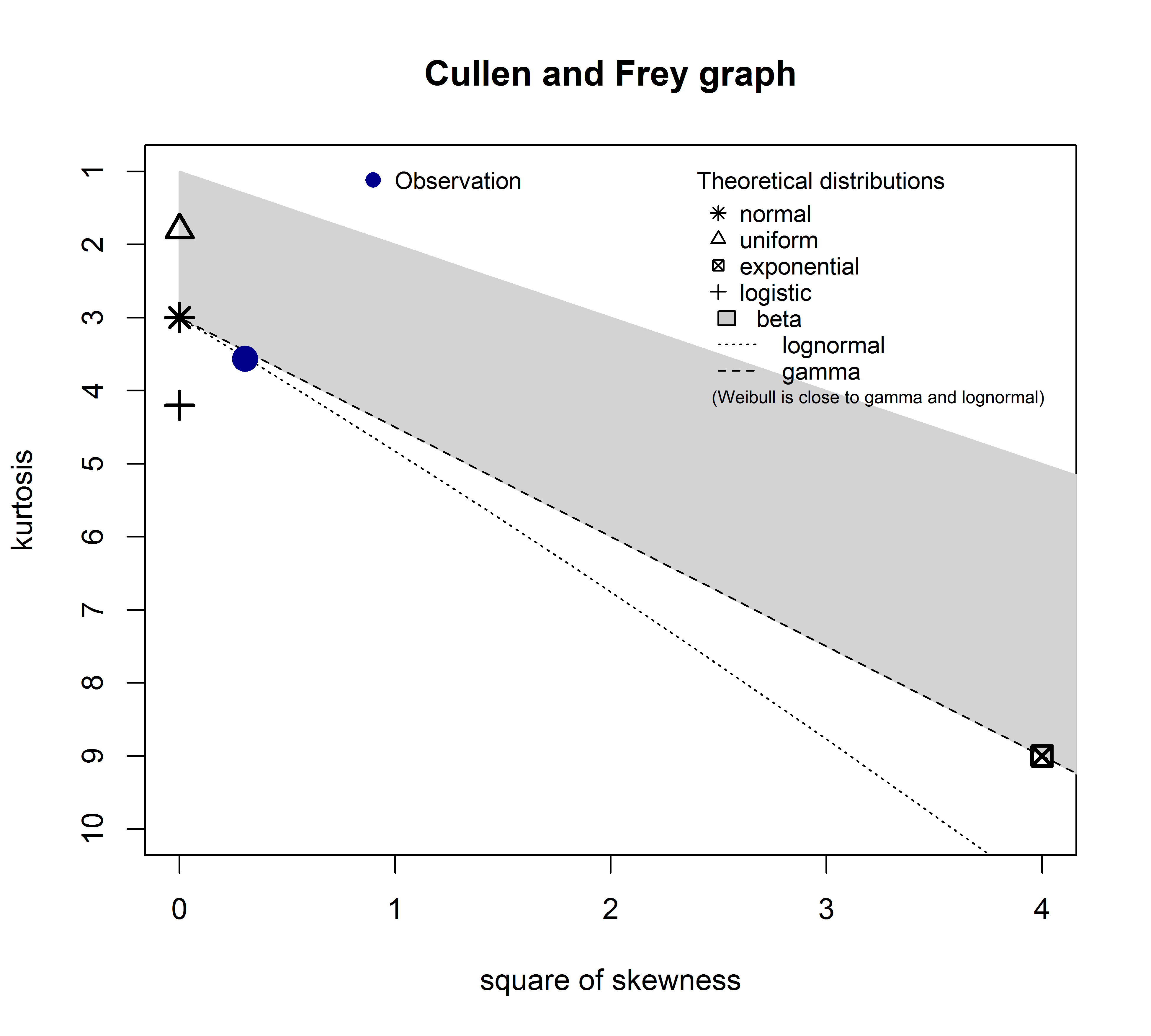
Descdist

The kurtosis and squared skewness of your sample are plotted as a blue point named "Observation". It seems that possible distributions include the Weibull, Lognormal and possibly the Gamma distribution.

Let's fit a Weibull distribution and a normal distribution:

fit.weibull <- fitdist(x, "weibull")
fit.norm <- fitdist(x, "norm")

Now inspect the fit for the normal:

plot(fit.norm)
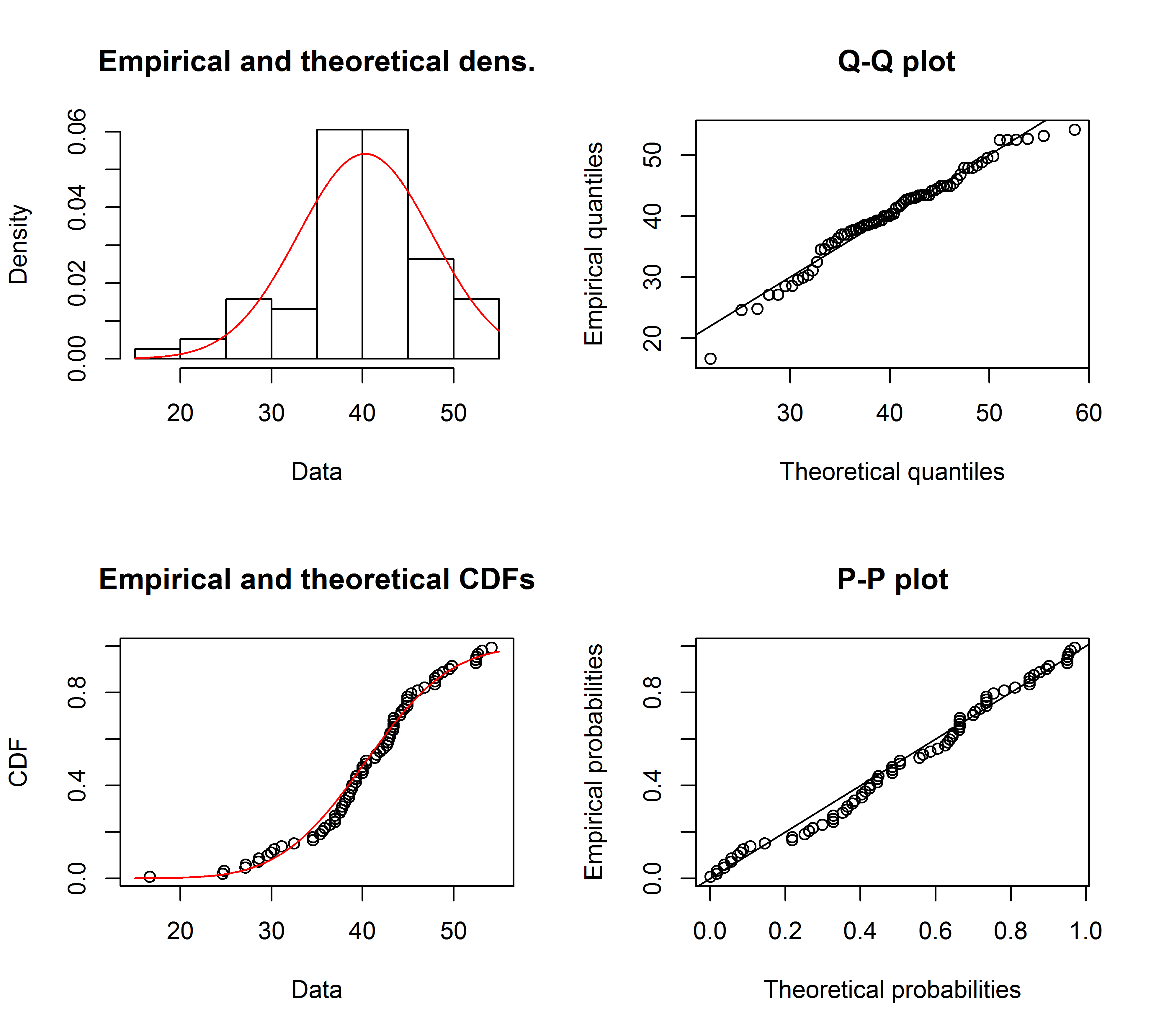
Normal fit

And for the Weibull fit:

plot(fit.weibull)
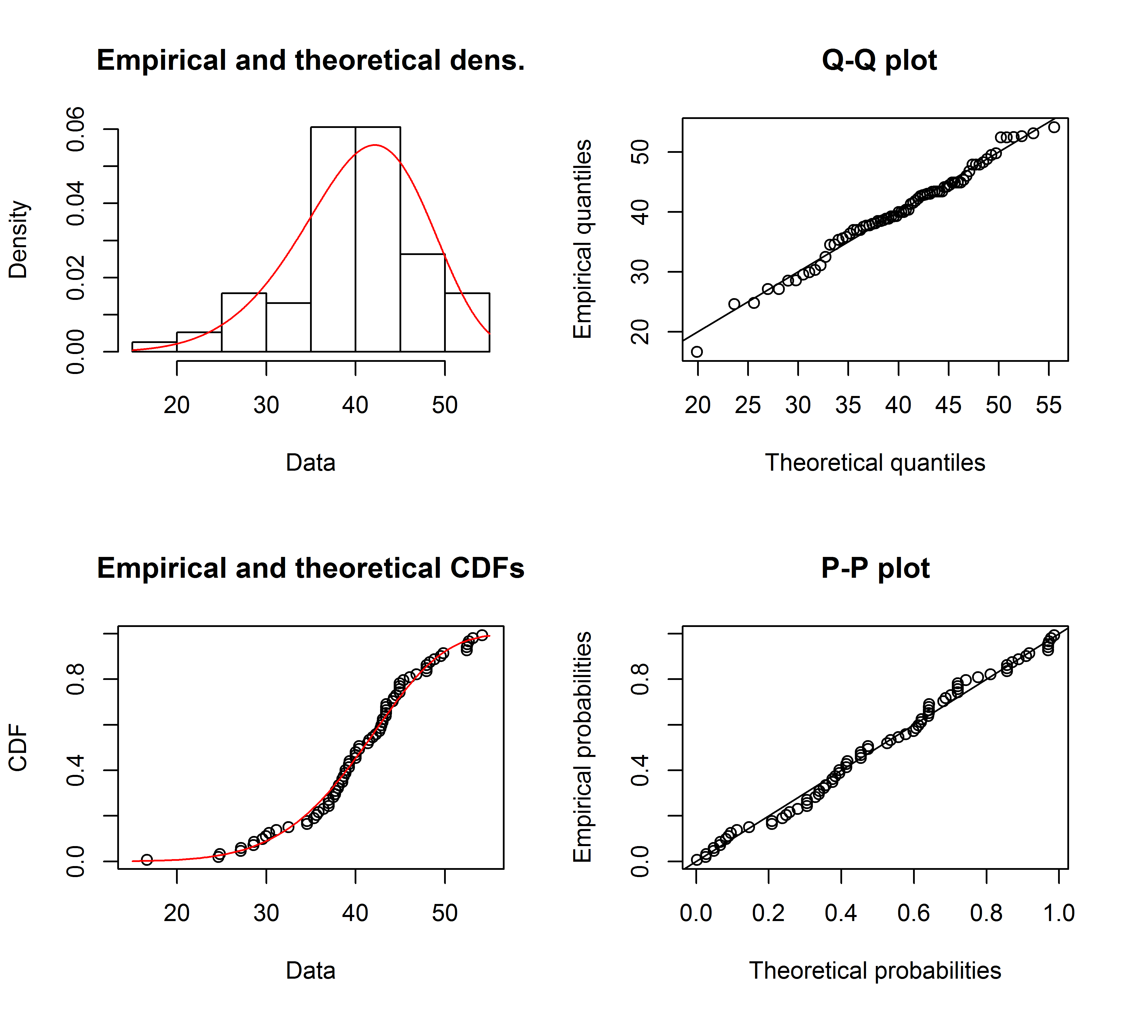
Weibull fit

Both look good but judged by the QQ-Plot, the Weibull maybe looks a bit better, especially in the tails. Correspondingly, the AIC of the Weibull fit is lower compared with the normal fit:

fit.weibull$aic
[1] 519.8537

fit.norm$aic
[1] 523.3079

Kolmogorov-Smirnov test simulation

I will use @Aksakal's procedure explained here to simulate the KS-statistic under the null.

n.sims <- 5e4

stats <- replicate(n.sims, {      
  r <- rweibull(n = length(x)
                , shape= fit.weibull$estimate["shape"]
                , scale = fit.weibull$estimate["scale"]
  )
  estfit.weibull <- fitdist(r, "weibull") # added to account for the estimated parameters
  as.numeric(ks.test(r
                     , "pweibull"
                     , shape= estfit.weibull$estimate["shape"]
                     , scale = estfit.weibull$estimate["scale"])$statistic
  )      
})

The ECDF of the simulated KS-statistics looks as follows:

plot(ecdf(stats), las = 1, main = "KS-test statistic simulation (CDF)", col = "darkorange", lwd = 1.7)
grid()
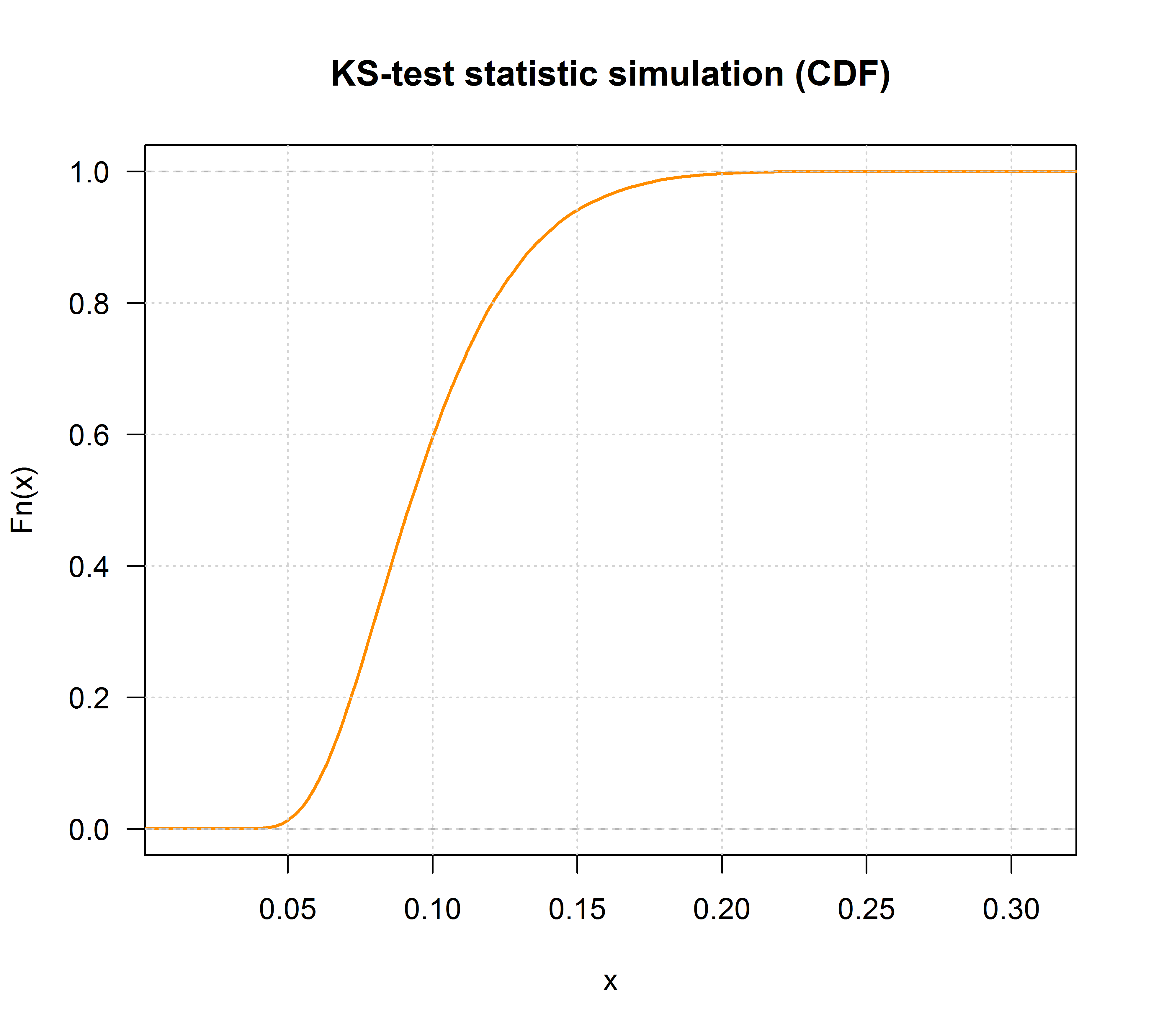
Simulated KS-statistics

Finally, our $p$-value using the simulated null distribution of the KS-statistics is:

fit <- logspline(stats)

1 - plogspline(ks.test(x
                       , "pweibull"
                       , shape= fit.weibull$estimate["shape"]
                       , scale = fit.weibull$estimate["scale"])$statistic
               , fit
)

[1] 0.4889511

This confirms our graphical conclusion that the sample is compatible with a Weibull distribution.

As explained here, we can use bootstrapping to add pointwise confidence intervals to the estimated Weibull PDF or CDF:

xs <- seq(10, 65, len=500)

true.weibull <- rweibull(1e6, shape= fit.weibull$estimate["shape"]
                         , scale = fit.weibull$estimate["scale"])

boot.pdf <- sapply(1:1000, function(i) {
  xi <- sample(x, size=length(x), replace=TRUE)
  MLE.est <- suppressWarnings(fitdist(xi, distr="weibull"))  
  dweibull(xs, shape=MLE.est$estimate["shape"],  scale = MLE.est$estimate["scale"])
}
)

boot.cdf <- sapply(1:1000, function(i) {
  xi <- sample(x, size=length(x), replace=TRUE)
  MLE.est <- suppressWarnings(fitdist(xi, distr="weibull"))  
  pweibull(xs, shape= MLE.est$estimate["shape"],  scale = MLE.est$estimate["scale"])
}
)   

#-----------------------------------------------------------------------------
# Plot PDF
#-----------------------------------------------------------------------------

par(bg="white", las=1, cex=1.2)
plot(xs, boot.pdf[, 1], type="l", col=rgb(.6, .6, .6, .1), ylim=range(boot.pdf),
     xlab="x", ylab="Probability density")
for(i in 2:ncol(boot.pdf)) lines(xs, boot.pdf[, i], col=rgb(.6, .6, .6, .1))

# Add pointwise confidence bands

quants <- apply(boot.pdf, 1, quantile, c(0.025, 0.5, 0.975))
min.point <- apply(boot.pdf, 1, min, na.rm=TRUE)
max.point <- apply(boot.pdf, 1, max, na.rm=TRUE)
lines(xs, quants[1, ], col="red", lwd=1.5, lty=2)
lines(xs, quants[3, ], col="red", lwd=1.5, lty=2)
lines(xs, quants[2, ], col="darkred", lwd=2)
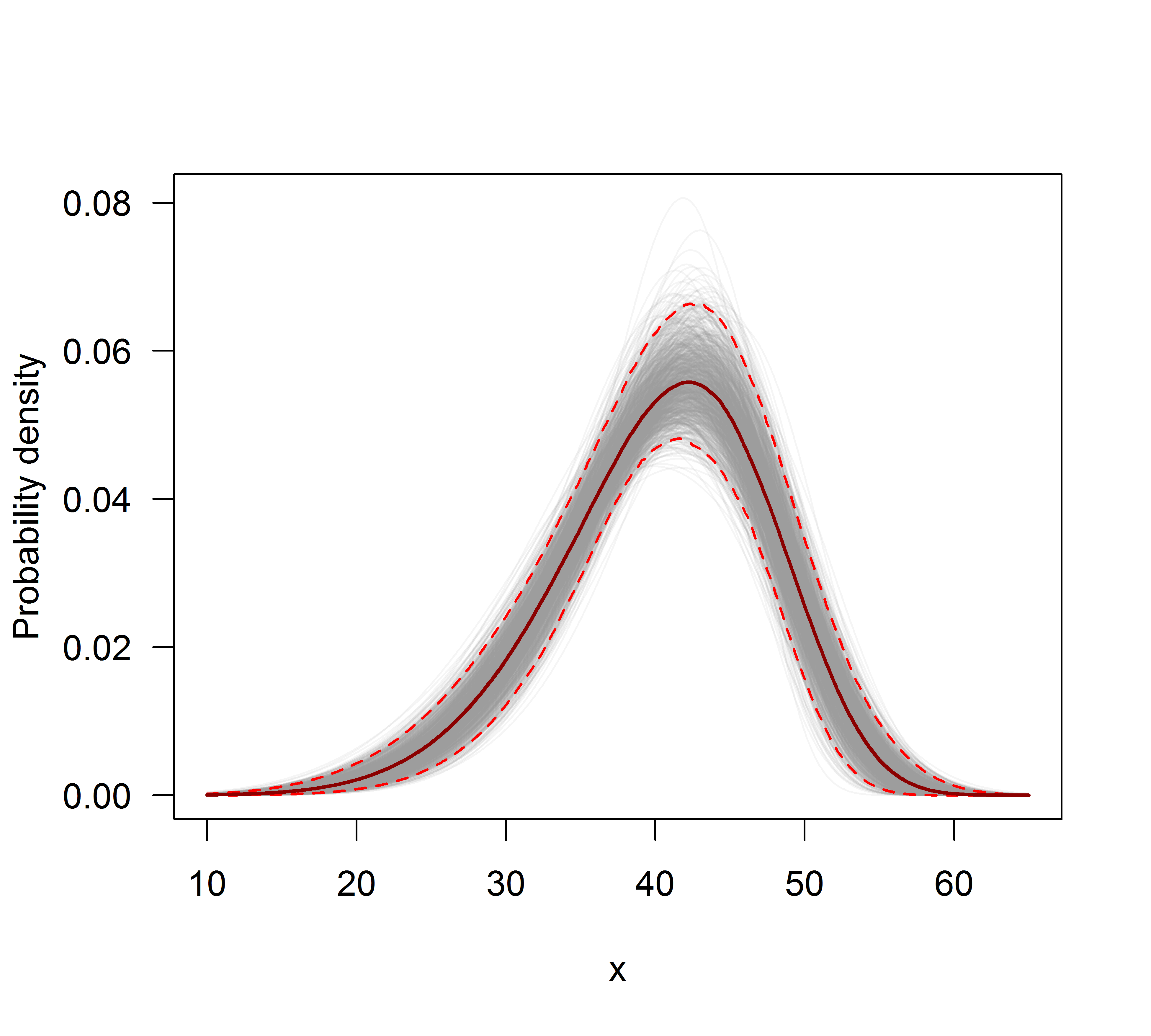
CI_Density

#-----------------------------------------------------------------------------
# Plot CDF
#-----------------------------------------------------------------------------

par(bg="white", las=1, cex=1.2)
plot(xs, boot.cdf[, 1], type="l", col=rgb(.6, .6, .6, .1), ylim=range(boot.cdf),
     xlab="x", ylab="F(x)")
for(i in 2:ncol(boot.cdf)) lines(xs, boot.cdf[, i], col=rgb(.6, .6, .6, .1))

# Add pointwise confidence bands

quants <- apply(boot.cdf, 1, quantile, c(0.025, 0.5, 0.975))
min.point <- apply(boot.cdf, 1, min, na.rm=TRUE)
max.point <- apply(boot.cdf, 1, max, na.rm=TRUE)
lines(xs, quants[1, ], col="red", lwd=1.5, lty=2)
lines(xs, quants[3, ], col="red", lwd=1.5, lty=2)
lines(xs, quants[2, ], col="darkred", lwd=2)
#lines(xs, min.point, col="purple")
#lines(xs, max.point, col="purple")
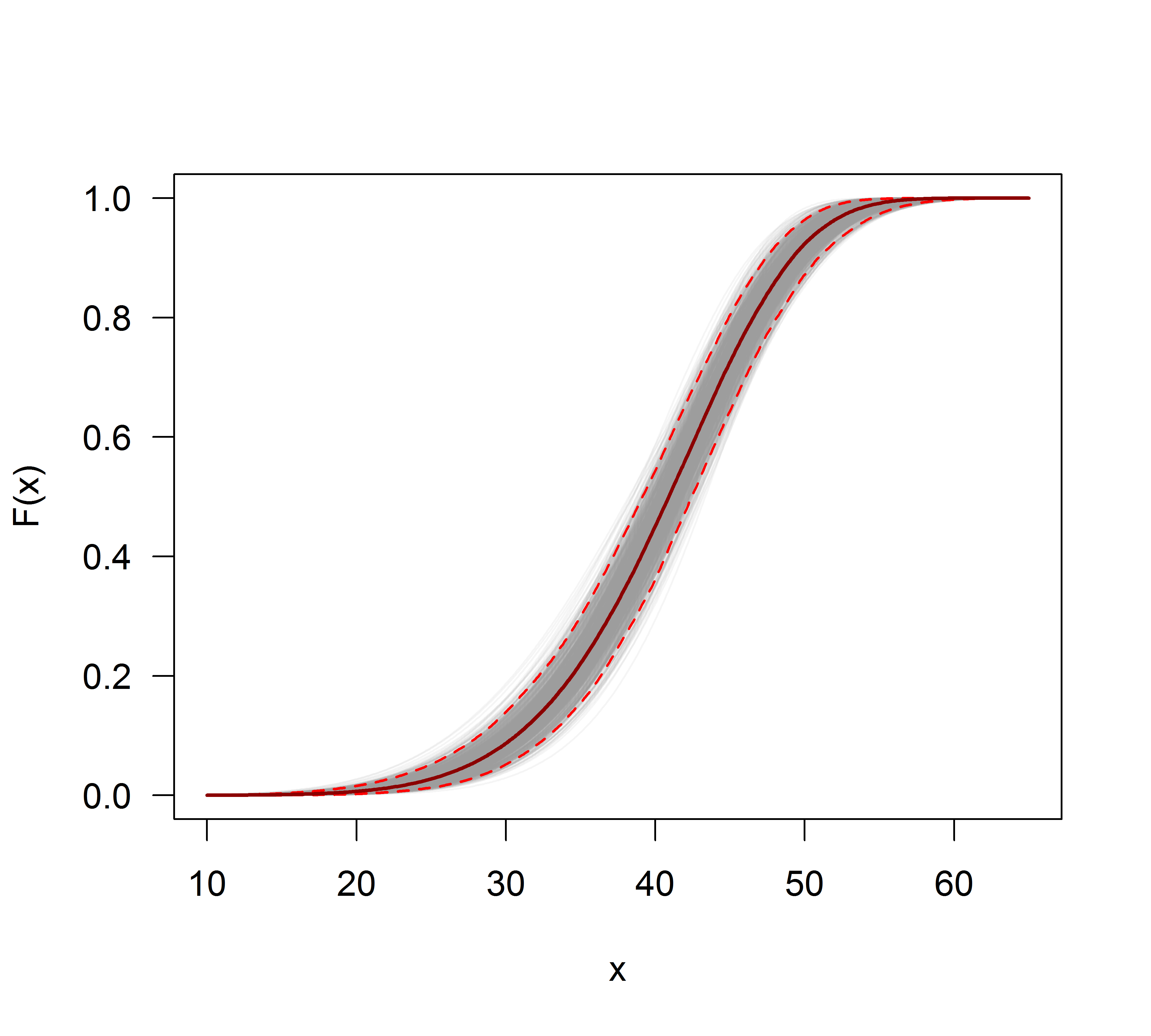
CI_CDF


Automatic distribution fitting with GAMLSS

The gamlss package for R offers the ability to try many different distributions and select the "best" according to the GAIC (the generalized Akaike information criterion). The main function is fitDist. An important option in this function is the type of the distributions that are tried. For example, setting type = "realline" will try all implemented distributions defined on the whole real line whereas type = "realsplus" will only try distributions defined on the real positive line. Another important option is the parameter $k$, which is the penalty for the GAIC. In the example below, I set the parameter $k = 2$ which means that the "best" distribution is selected according to the classic AIC. You can set $k$ to anything you like, such as $\log(n)$ for the BIC.

library(gamlss)
library(gamlss.dist)
library(gamlss.add)

x <- c(37.50,46.79,48.30,46.04,43.40,39.25,38.49,49.51,40.38,36.98,40.00,
       38.49,37.74,47.92,44.53,44.91,44.91,40.00,41.51,47.92,36.98,43.40,
       42.26,41.89,38.87,43.02,39.25,40.38,42.64,36.98,44.15,44.91,43.40,
       49.81,38.87,40.00,52.45,53.13,47.92,52.45,44.91,29.54,27.13,35.60,
       45.34,43.37,54.15,42.77,42.88,44.26,27.14,39.31,24.80,16.62,30.30,
       36.39,28.60,28.53,35.84,31.10,34.55,52.65,48.81,43.42,52.49,38.00,
       38.65,34.54,37.70,38.11,43.05,29.95,32.48,24.63,35.33,41.34)

fit <- fitDist(x, k = 2, type = "realplus", trace = FALSE, try.gamlss = TRUE)

summary(fit)

*******************************************************************
Family:  c("WEI2", "Weibull type 2") 

Call:  gamlssML(formula = y, family = DIST[i], data = sys.parent()) 

Fitting method: "nlminb" 


Coefficient(s):
             Estimate  Std. Error  t value   Pr(>|t|)    
eta.mu    -24.3468041   2.2141197 -10.9962 < 2.22e-16 ***
eta.sigma   1.8661380   0.0892799  20.9021 < 2.22e-16 ***

According to the AIC, the Weibull distribution (more specifically WEI2, a special parametrization of it) fits the data best. The exact parameterization of the distribution WEI2 is detailed in this document on page 279. Let's inspect the fit by looking at the residuals in a worm plot (basically a de-trended Q-Q-plot):
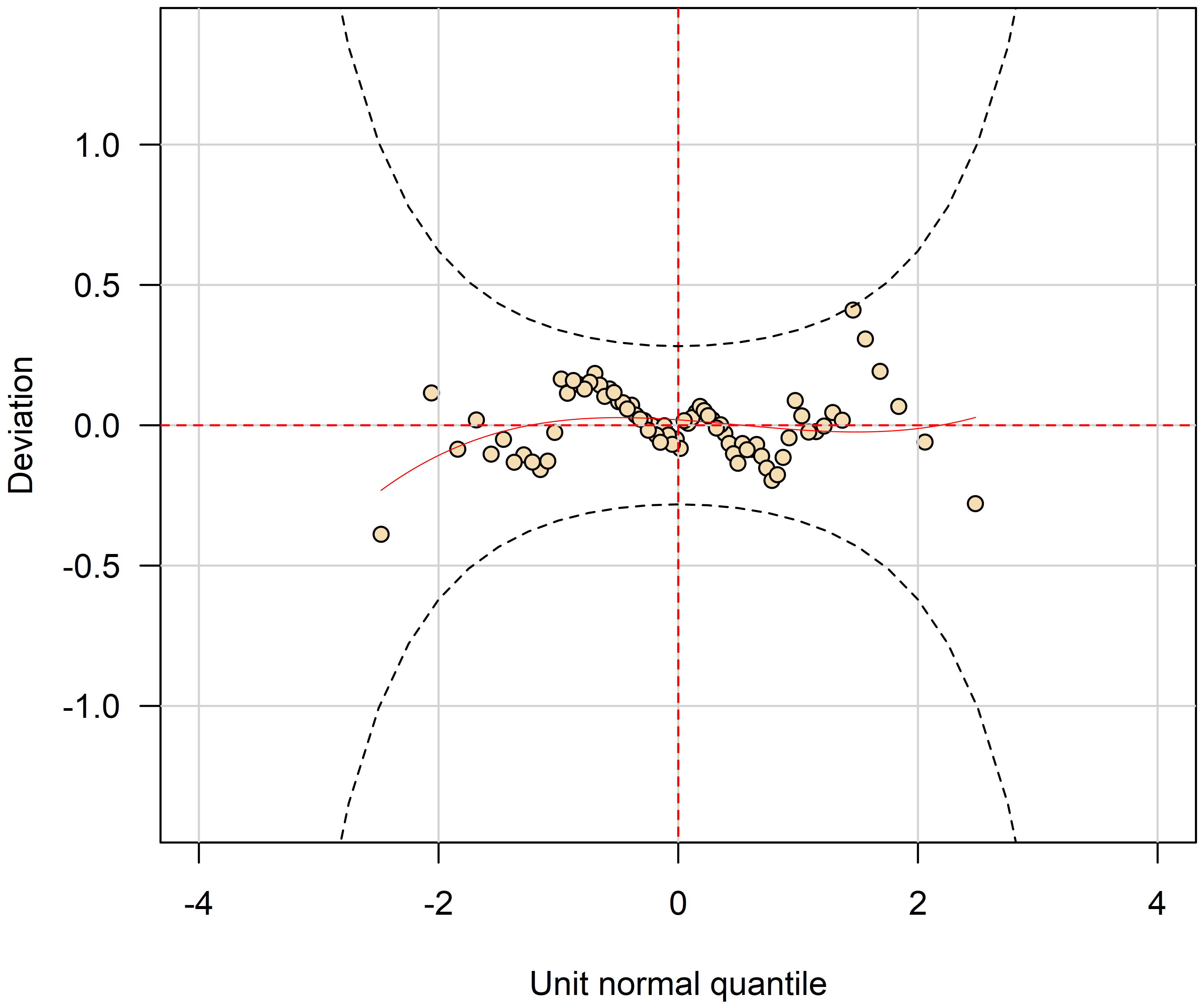
WormPlot

We expect the residuals to be close to the middle horizontal line and 95% of them to lie between the upper and lower dotted curves, which act as 95% pointwise confidence intervals. In this case, the worm plot looks fine to me indicating that the Weibull distribution is an adequate fit.

$\endgroup$
12
  • 4
    $\begingroup$ +1 Nice analysis. One question, though. Does positive conclusion on compatibility with a particular major distribution (Weibull, in this case) allows to rule out a possibility of a mixture distribution's presence? Or we need to perform a proper mixture analysis and check GoF to rule out that option? $\endgroup$ Commented Jan 8, 2015 at 19:00
  • 23
    $\begingroup$ @AleksandrBlekh It is impossible to have enough power to rule out a mixture: when the mixture is of two almost identical distributions it cannot be detected and when all but one component have very small proportions it cannot be detected, either. Typically (in the absence of a theory which might suggest a distributional form), one fits parametric distributions in order to achieve parsimonious approximate descriptions of data. Mixtures are none of those: they require too many parameters and are too flexible for the purpose. $\endgroup$
    – whuber
    Commented Jan 8, 2015 at 19:04
  • 4
    $\begingroup$ @whuber: +1 Appreciate your excellent explanation! $\endgroup$ Commented Jan 8, 2015 at 19:25
  • 2
    $\begingroup$ @Lourenco I looked at the Cullen and Fey graph. The blue point denotes our sample. You see that the point is close to the lines of the Weibull, Lognormal and Gamma (which is between Weibull and Gamma). After fitting each of those distributions, I compared the goodness-of-fit statistics using the function gofstat and the AIC. There isn't a consensus about what the best way to determine the "best" distribution is. I like graphical methods and the AIC. $\endgroup$ Commented Jun 23, 2017 at 17:33
  • 1
    $\begingroup$ @Lourenco Do you mean the lognormal? The logistic distribution (the "+" sign) is quite a bit away from the observed data. The lognormal would also be a candidate I'd normally look at. For this tutorial, I've chosen to not show it in order to keep the post short. The lognormal shows a worse fit compared to both the Weibull and Normal distribution. The AIC is 537.59 and the graphs also don't look too good. $\endgroup$ Commented Jun 26, 2017 at 19:19
20
$\begingroup$

Plots are mostly a good way to get a better idea of what your data looks like. In your case I would recommend plotting the empirical cumulative distribution function (ecdf) against the theoretical cdfs with the parameters you got from fitdistr().

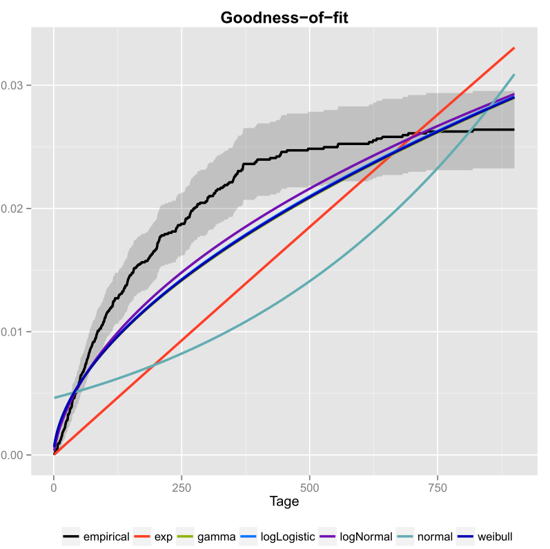
I did that once for my data and also included the confidence intervals. Here is the picture I got using ggplot2().

enter image description here

The black line is the empirical cumulative distribution function and the colored lines are cdfs from different distributions using parameters I got using the Maximum Likelihood method. One can easily see that the exponential and normal distribution are not a good fit to the data, because the lines have a different form than the ecdf and lines are quite far away from the ecdf. Unfortunately the other distribtions are quite close. But I would say that the logNormal line is the closest to the black line. Using a measure of distance (for example MSE) one could validate the assumption.

If you only have two competing distributions (for example picking the ones that seem to fit best in the plot) you could use a Likelihood-Ratio-Test to test which distributions fits better.

$\endgroup$
9
  • 25
    $\begingroup$ Welcome to CrossValidated! Your answer might be more useful if you could edit it to include (a) the code you used to produce the graphic, and (b) how one would read the graphic. $\endgroup$ Commented Jan 8, 2015 at 10:49
  • 2
    $\begingroup$ What is being plotted there? Is that some sort of exponentiality-plot? $\endgroup$
    – Glen_b
    Commented Jan 8, 2015 at 11:00
  • 1
    $\begingroup$ But how do you decide which distribution fits your data best? Only according to the graphic I couldn't tell you whether logNormal or weibull fits your data best. $\endgroup$
    – tobibo
    Commented Jan 8, 2015 at 11:27
  • 4
    $\begingroup$ If you want to create a pseudo-random numbers generator why not use the empirical cdf? Do you want to draw numbers that go beyond your observed distribution? $\endgroup$ Commented Jan 8, 2015 at 12:14
  • 7
    $\begingroup$ Taking your graph at face value, it would appear that none of your candidate distributions fit the data well at all. Also, your ecdf appears to have a horizontal asymptote at less than 0.03 which doesn't make sense, so I'm not sure that it really is an ecdf in the first place. $\endgroup$
    – Hong Ooi
    Commented Jan 8, 2015 at 15:56
3
$\begingroup$

Following up on the brief answer by @Isr727, I like their suggestion of univariateML best because it provides an automatic solution for this challenge. The other answers are great for analyzing the "best" solution in-depth, but univariateML provides tools to make a good automatic choice, which is essential when the generation of random variables is embedded in a more complex workflow procedure (as is my use case).

univariateML provides a model_select function that automatically tests the fit of many different distributions and then selects the best fit based on AIC (default), BIC, or log likelihood. You can see all the distributions that it tests listed in the univariateML_models object:

install.packages('univariateML')
univariateML::univariateML_models
# [1] "beta"       "betapr"     "cauchy"     "exp"        "gamma"      "ged"        "gumbel"    
# [8] "invgamma"   "invgauss"   "invweibull" "kumar"      "laplace"    "lgamma"     "llogis"    
# [15] "lnorm"      "logis"      "logitnorm"  "lomax"      "naka"       "norm"       "pareto"    
# [22] "power"      "rayleigh"   "sged"       "snorm"      "sstd"       "std"        "unif"      
# [29] "weibull"   

With OP's data, a simple call to model_select quickly identifies Weibull as the best fit:

mydata_dist <- univariateML::model_select(mydata)
mydata_dist
# Maximum likelihood estimates for the Weibull model 
# shape   scale  
# 6.463  43.247  

It is reassuring to see that model_select automatically selects the same distribution as did the other question answers with their careful, in-depth analysis.

Going further, the rml function easily meets OP's original need of generating a random variable based on any of the supported distributions. In particular, that function can take the output distribution from model_select to easily generate a suitable random variable:

set.seed(0)
rand_var <- univariateML::rml(
  n = length(mydata),
  obj = univariateML::model_select(mydata)
)
rand_var
# [1] 30.69403 45.17789 43.17032 39.50521 30.10888 46.51431 30.61130 27.75671 37.73572 38.39577
# [11] 50.67124 46.41912 47.09237 37.16414 42.95326 35.14390 40.90521 36.46145 20.53920 43.02688
# [21] 34.93626 28.50062 46.28393 37.92894 48.41834 45.14394 42.91692 54.22219 42.98430 31.89081
# [31] 43.75159 41.18899 38.98698 40.98092 46.86558 33.43428 37.57117 34.45998 48.94790 36.31615
# [41] 42.46356 33.64355 38.02563 34.78342 39.88153 40.31705 34.60113 53.07833 41.27679 36.10758
# [51] 37.03619 41.26975 32.22730 41.98169 45.59530 50.28462 49.22192 44.19967 40.52181 37.70995
# [61] 42.54349 29.85506 44.62989 41.60461 43.89876 37.94582 45.32740 41.25300 35.23875 49.75394
# [71] 31.65817 43.77515 33.02562 43.63492 43.87316 41.29269
$\endgroup$
1
$\begingroup$

Apart from the above-mentioned ways, another approach is to fit as many distributions as you can and estimate their parameters, then compare the AIC and select the best model that fits your data. You dont need to do that on your own, there are several packages available in R and python. In python, Fitter may be used, and in R, univariateML seems nice to me.

You can have a look at some examples of fitting different distributions and finding the best one using univariateML here and here.

$\endgroup$

Not the answer you're looking for? Browse other questions tagged or ask your own question.