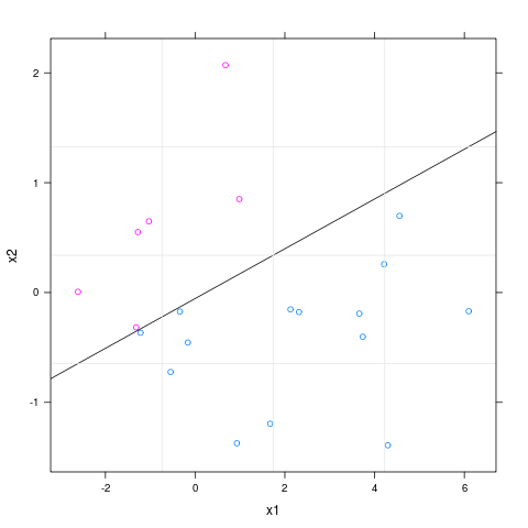
I made a logistic regression model using glm in R. I have two independent variables. How can I plot the decision boundary of my model in the scatter plot of the two variables. For example, how can I plot a figure like here.
2 Answers
set.seed(1234)

x1 <- rnorm(20, 1, 2)
x2 <- rnorm(20)

y <- sign(-1 - 2 * x1 + 4 * x2 )

y[ y == -1] <- 0

df <- cbind.data.frame( y, x1, x2)

mdl <- glm( y ~ . , data = df , family=binomial)

slope <- coef(mdl)[2]/(-coef(mdl)[3])
intercept <- coef(mdl)[1]/(-coef(mdl)[3])

library(lattice)
xyplot( x2 ~ x1 , data = df, groups = y,
   panel=function(...){
       panel.xyplot(...)
       panel.abline(intercept , slope)
       panel.grid(...)
       })

I must remark that perfect separation occurs here, therefore the glm function gives you a warning. But that is not important here as the purpose is to illustrate how to draw the linear boundary and the observations colored according to their covariates.
-
$\begingroup$ I hope I am not old fashioned if I use lattice :-) $\endgroup$ Commented Jan 13, 2011 at 2:47
-
2$\begingroup$ I also hope that if this is a HW problem, you will not simply copy paste. $\endgroup$ Commented Jan 13, 2011 at 2:54
-
$\begingroup$ Thanks. This is not a HW question and the answer is helpful for me to understand my model. $\endgroup$– user2755Commented Jan 13, 2011 at 4:25
-
-
1$\begingroup$ Can someone explain me the logic behind the slope and intercept? (regarding the logistic model) $\endgroup$– FernandoCommented Jan 9, 2013 at 12:29
Wanted to address the question in comment to the accepted answer above from Fernando: Can someone explain the logic behind the slope and intercept?
The hypothesis for logistics regression takes the form of:
$$h_{\theta} = g(z)$$
where, $g(z)$ is the sigmoid function and where $z$ is of the form:
$$z = \theta_{0} + \theta_{1}x_{1} + \theta_{2}x_{2}$$
Given we are classifying between 0 and 1, $y = 1$ when $h_{\theta} \geq 0.5$ which given the sigmoid function is true when:
$$\theta_{0} + \theta_{1}x_{1} + \theta_{2}x_{2} \geq 0$$
the above is the decision boundary and can be rearranged as:
$$x_{2} \geq \frac{-\theta_{0}}{\theta_{2}} + \frac{-\theta_{1}}{\theta_{2}}x_{1}$$
This is an equation in the form of $y = mx + b$ and you can see then why $m$ and $b$ are calculated the way they are in the accepted answer
-
2$\begingroup$ Good explanation accompanying the answer above! $\endgroup$– AugustinCommented Dec 29, 2015 at 11:04
-
$\begingroup$ If we classify $y=1$ based on $h_θ ≥ t$ for a general $t$ between 0 and 1, we have $θ_0 + θ_1 x_1 + θ_2 x_2 ≥ \text{log odds}(t)$. $\endgroup$– husBCommented Dec 6, 2023 at 10:32
