Moderation coefficient in linear mixed models SPSS - interpretation

Question

My model:

IV: extroversion (5 point likert) Moderator: Comepetence (values 1-5) DV: Offer (values 5 to 15)

Hypothesis: The negative relationship between Extroversion and offer is moderated by competence, such that higher competence weakens the negative relationship.

My output: (significance cut-off value is .1, not .05 in my case)

There is no significant negative direct effect between extroversion and competenece.

The extroversion*comeptence interaction effect is significant, but the coefficient is positive. Does this support my hypothesis or it means the complete opposite (that higher competence trust intensifies the negative relationship between extroversion and offer).

Please help me i am very confused on what the results mean.

Answer 1

Here's a quick example of interpreting and visualizing a continuous x continuous interaction:

#create some data with similar properties as your data

set.seed(123)
Ex<-rnorm(1:100)
Comp<-rnorm(1:100)
Offer<-3+(-.7*x)+(-1*z)+(0.5*(x*z))+rnorm(100)
example_df<-data.frame(Ex,Comp,Offer)
model<-lm(Offer ~ Ex*Comp, data=example_df)
summary(model)

Call:
lm(formula = Offer ~ Ex * Comp, data = example_df)

Residuals:
    Min      1Q  Median      3Q     Max 
-1.8719 -0.6777 -0.1086  0.5897  2.3166 

Coefficients:
            Estimate Std. Error t value Pr(>|t|)    
(Intercept)  3.14098    0.09578  32.795  < 2e-16 ***
Ex          -0.79281    0.10834  -7.318 7.65e-11 ***
Comp        -0.96566    0.09881  -9.772 4.58e-16 ***
Ex:Comp      0.65911    0.11449   5.757 1.03e-07 ***
---
Signif. codes:  0 ‘***’ 0.001 ‘**’ 0.01 ‘*’ 0.05 ‘.’ 0.1 ‘ ’ 1

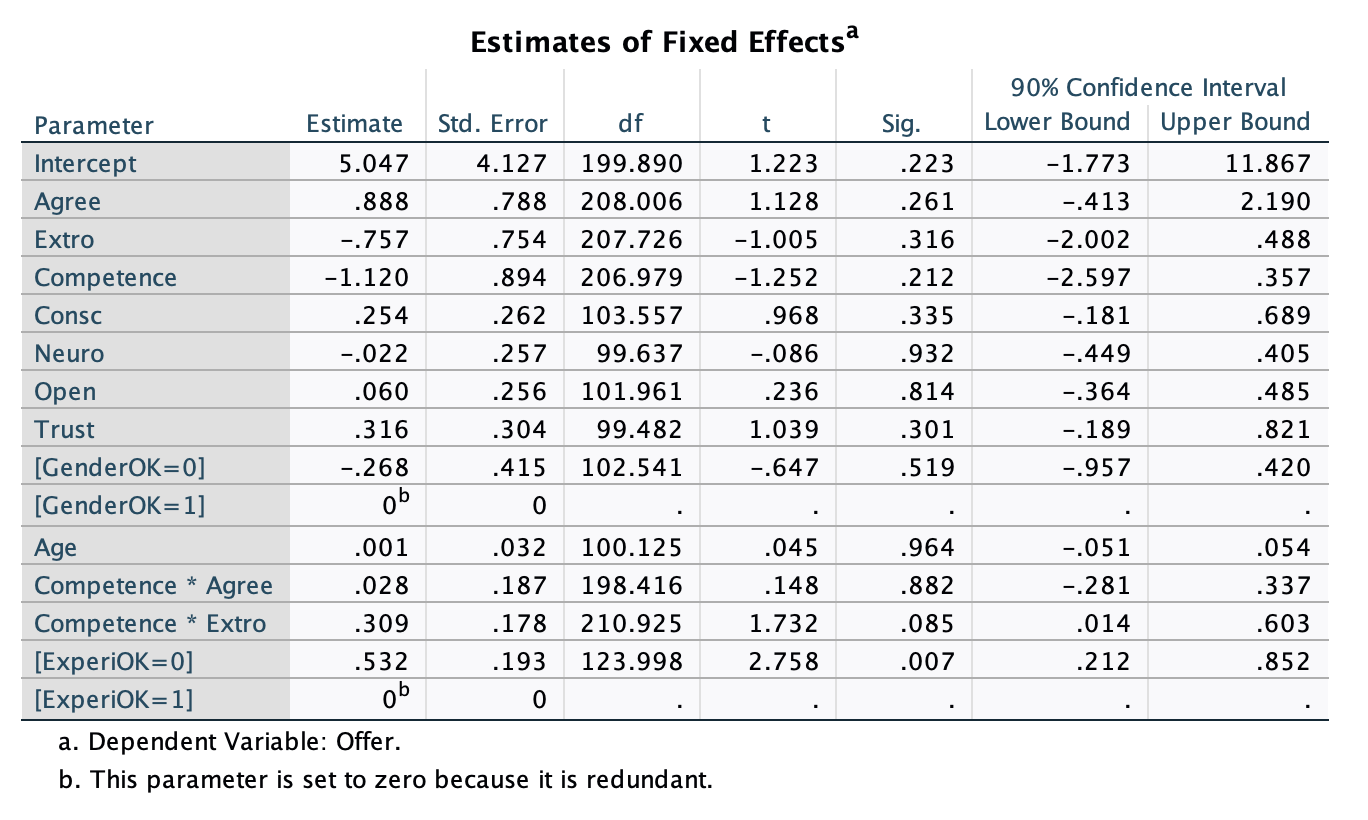
So, here, the coefficients mimic your relevant coefficients (the fact that you have a multilevel model and mine is a single-level one does not matter for the example).

Then, we can visualize the interaction:

#First, let's get interesting values for Competence:
mean(example_df$Comp) #mean of Comp
-0.1075468
mean(example_df$Comp)-sd(example_df$Comp) #mean - 1sd of Comp
-1.074533
mean(example_df$Comp)+sd(example_df$Comp) #mean + 1 sd of Comp
0.8594398

library(sjPlot)
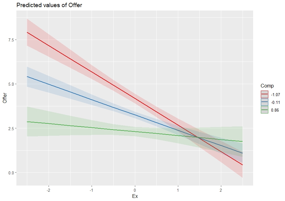
plot_model(model, type="pred", terms=c("Ex", "Comp[-1.07, .11, 0.86]"))

As you can see from the image, when Competence is low or average, the effect of Extraversion is pretty strongly negative, but when Competence is high (+1 sd), the effect of Extraversion is only slightly negative.