Two way anova or paired t-tests

Question

i am looking to see if there is a difference in dissolved oxygen levels between pool surface (S) and bottom (B) samples at four sites (an up and downstream site in two creeks). There are 3 replicate readings at each site, each replicate has a surface and bottom reading at the same location (paired surface and bottom readings). The sites and replicates were sampled on two separate occasions (Period).

I'm interested in finding out if there are higher dissolved oxygen levels at the surface compared to bottom samples, but also if there are also interactions between period and site. Is a three-way anova with Period (2 level factor), site (4 level factor) and depth (2 level factor) appropriate? Or would paired t-tests be more suitable, grouped for sites (pooling both periods' data) for analysis of within site differences?

Thankyou in advance

Period	Site	S	B
1	LCU	100.1	70.8
1	LCU	99.3	60.6
1	LCU	95.5	66.0
1	LCD	90.3	55.6
1	LCD	85.8	51.0
1	LCD	90.6	51.8
1	MCU	85.5	90.0
1	MCU	86.9	86.0
1	MCU	85.4	94.0
1	MCD	92.9	45.0
1	MCD	88.6	56.9
1	MCD	89.4	70.1
2	LCU	70.0	20.0
2	LCU	66.4	28.5
2	LCU	61.3	29.4
2	LCD	55.6	55.1
2	LCD	55.8	48.2
2	LCD	57.8	48.1
2	MCU	54.0	52.1
2	MCU	53.2	53.3
2	MCU	53.3	51.1
2	MCD	40.0	18.0
2	MCD	41.0	28.9
2	MCD	44.9	26.4

Answer 1

You can use a repeated measures ANOVA, or mixed model to account for the replicates at the same time and location for bottom and surface measurements.

To do this, I made two changes to your data:

• Convert it to long format. This is what most statistical software expects for this type of model.
• Split the Site variable into Creek and Direction (upstream or downstream). This allows you to choose whether or not to include an interaction between the two, providing more flexibility.

require("glmmTMB")
LMM <- glmmTMB(Oxygen ~ Period * Creek + Direction + Type + (1 | Replicate), 
               data = Long)
summary(LMM)

Output:

 Family: gaussian  ( identity )
Formula:          Oxygen ~ Period * Creek + Direction + Type + (1 | Replicate)
Data: Long

     AIC      BIC   logLik deviance df.resid 
   375.9    390.9   -180.0    359.9       40 

Random effects:

Conditional model:
 Groups    Name        Variance  Std.Dev. 
 Replicate (Intercept) 1.993e-07 4.464e-04
 Residual              1.057e+02 1.028e+01
Number of obs: 48, groups:  Replicate, 24

Dispersion estimate for gaussian family (sigma^2):  106 

Conditional model:
                Estimate Std. Error z value Pr(>|z|)    
(Intercept)       61.625      3.635  16.952  < 2e-16 ***
Period2          -26.767      4.198  -6.377 1.81e-10 ***
CreekMC            4.442      4.198   1.058  0.29000    
DirectionU         9.371      2.968   3.157  0.00159 ** 
TypeSurface       20.279      2.968   6.832 8.37e-12 ***
Period2:CreekMC  -11.108      5.936  -1.871  0.06132 .  
---
Signif. codes:  0 ‘***’ 0.001 ‘**’ 0.01 ‘*’ 0.05 ‘.’ 0.1 ‘ ’ 1

From the output, you can see that the variance between replicates is very small compared to the residual variance, so omitting the random effect for Replicate and using lm will give practically identical results.

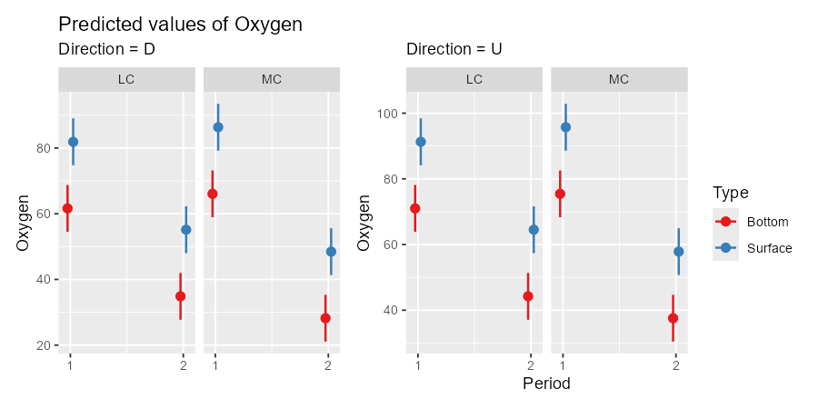
Here is a visualization that summarizes the model, using the great package sjPlot:

require("sjPlot")
plot_model(LMM, type = "pred", terms = c("Period", "Type", "Creek", "Direction"))

---

Code

DF <- read.csv("CV_652520.csv")
DF$Direction <- factor(substr(DF$Site, 3, 3))
DF$Creek     <- factor(substr(DF$Site, 1, 2))

Long <- data.frame(
  Period    = factor(rep(DF$Period, 2)),
  Creek     = rep(DF$Creek, 2),
  Direction = rep(DF$Direction, 2),
  Oxygen    = c(DF$S, DF$B),
  Type      = factor(rep(c("Surface", "Bottom"), each = nrow(DF))),
  Replicate = factor(rep(1:nrow(DF), 2))
)

require("glmmTMB")
LMM <- glmmTMB(Oxygen ~ Period * Creek + Direction + Type + (1 | Replicate), 
               data = Long)
summary(LMM)

require("sjPlot")
plot_model(LMM, type = "pred", terms = c("Period", "Type", "Creek", "Direction"))