In what follows, please remember that I am showing an approach, not the approach. The approach depends on assumptions, much of which I can not validate (nor do I have the wish to validate thoroughly since doing so might require I border on consulting, which I do not wish to do frankly).
Do you have any suggestions which method will be reliable in practice?
Assuming for now that there is no correlation between sessions from the same user (almost certainly and demonstrably false, but we can return to this in a moment), and that number of sessions per user is independent of exposure, and that average revenue per converted session is independent of conversion rate in the prior model, I think a Bayesian hurdle model is a good first start.
Why hurdle? The revenue observation is only observed once the user "jumps the hurdle" of intending to purchase. So there are two distinct processes to model: the conversion probability, and the amount of revenue obtained from the session. As you allude to in one of your comments, a decrease in conversion rate can be made up for by a suitable increase in revenue, and vice versa.
Why Bayesian? Two reasons: i) Model checks are going to be very important here because revenue data can behave in pathological ways, and ii) We can use the model based approach as described in Imbens and Rubin's "Causal Inference for statistics, social, and medical sciences".
Model
Suppose that the total revenue (we'll get to revenue per session) in arm $k$ is given by $y_k$, and that in arm $k$ a total $n_k$ of $N_k$ sessions result in a purchase. Then we can model $y_k$ as
$$ y_k \sim \operatorname{Binomial}(N_k, \theta_k) \times \operatorname{Gamma}(n_k, 1/\lambda_k) $$
with appropriate priors. Here:
- $\theta_k$ is the rate at which sessions result in a purchase.
- The gamma distribution is parameterized in terms of shape and rate, so that the expected total revenue from sessions resulting in a purchase is $n_k \lambda_k$.
- This means $\lambda_k$ is interpreted as the expected revenue from a single converted session.
How can we use this to determine the average revenue per session? As mentioned, we can use the model based approach from Imbens and Rubin. In short, we can
- Assume we observe some amount of new sessions.
- Use the model to estimate counterfactual revenue for each session
- Estimate the mean revenue in each session, and
- Average our estimates over many MCMC draws from the posterior.
Simulation
Let's simulate some simple data in R. I'll generate 1 million sessions from two hypothetical populations -- one where all are treated, and one where all are control. Then, I will sample 100, 000 sessions from these populations. The conversion rate $\theta_k$ is the same in both populations, but the expected revenue from a converted session is higher by \$2 (so uniform between 42 and 82) in the treated population. I'm going to summarize the data so that we know: How many users did not convert, how many did convert, and what the total revenue from the converted sessions was.
library(tidyverse)
library(cmdstanr)
#> This is cmdstanr version 0.7.1
#> - CmdStanR documentation and vignettes: mc-stan.org/cmdstanr
#> - CmdStan path: /Users/demetripananos/.cmdstan/cmdstan-2.34.1
#> - CmdStan version: 2.34.1
#>
#> A newer version of CmdStan is available. See ?install_cmdstan() to install it.
#> To disable this check set option or environment variable CMDSTANR_NO_VER_CHECK=TRUE.
library(tidybayes)

set.seed(0)
N <- 1000000
pop1 <- runif(N, 40, 80) * rbinom(N, 1, 0.6)
pop2 <- runif(N, 42, 82) * rbinom(N, 1, 0.6)

n <- 100000
x1 <- tibble(arm = "A", y = sample(pop1, size=n))
x2 <- tibble(arm = "B", y = sample(pop2, size=n))
d <- bind_rows(x1, x2)

md <- d %>%
     mutate(paid = if_else(y==0, 0, 1),
            arm = factor(arm)) %>%
     group_by(arm) %>%
     summarise(
       Nn = sum(y>0),
       y = sum(y),
       N = n(),
     )


md
#> # A tibble: 2 × 4
#>   arm      Nn        y      N
#>   <fct> <int>    <dbl>  <int>
#> 1 A     60074 3607691. 100000
#> 2 B     59768 3707771. 100000
Created on 2024-08-29 with reprex v2.0.2
You can verify that B has more revenue per session at about \$37 per session (which happens to be the average revenue per converting session -- \$60 -- multiplied by the conversion probability -- 60%).
Now, we will write a stan model to estimate the parameters from the data and do the simulation. The model looks like
stan_code <- '
data{
  int n;
  int n_arm;
  array[n] int Nn;
  array[n] int arm;
  array[n] real y;
  array[n] int N;
  int ng;

}
parameters{
  // Spending rate per session
  array[n_arm] real <lower=0> lambda;

  // Probability of spending
  array[n_arm] real <lower=0, upper=1> theta;
}
model{
  target += cauchy_lpdf(lambda|0, 1);
  target += beta_lpdf(theta | 1, 1);
  for(i in 1:n){
  target += binomial_lpmf( Nn[i]| N[i], theta[arm[i]]);
  target += gamma_lpdf(y[i]| Nn[i], lambda[arm[i]]);
  }

}

generated quantities{

  array[n_arm] real rev_per_session;

  {

  array[n_arm, ng] real yppc;

    for(i in 1:n_arm){
      for(j in 1:ng){
        yppc[i, j] = gamma_rng(1.0, lambda[i]) * binomial_rng(1, theta[i]);
      }
      rev_per_session[i] = sum(yppc[i, ]);
    }
  }

}

'
We'll now fit the model to the data
model <- stan_code %>%
         write_stan_file() %>%
         cmdstan_model()


stan_data <- compose_data(d)
stan_data$ng <- n


fit <- model$sample(stan_data, parallel_chains = 4)
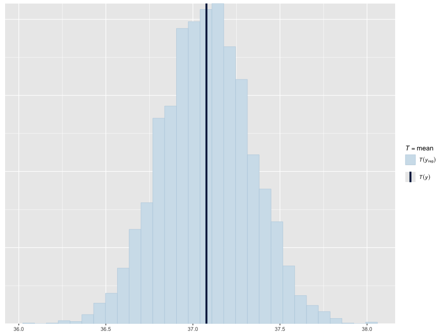
We can check that the model produces reasonable estimates with some other posterior predictive checks. Here, I will plot the estimated total revenue from each of the 100,000 sessions for B. The vertical line indicates the observed value, while the histogram are the model predictions. I will leave you to determine if (and in what way) the model predictions are deficient, but for now they predict that the observed revenue per session of 37 is among the most predicted quantities.
yppc <- posterior::as_draws_matrix(fit$draws('rev_per_session'))


bayesplot::ppc_stat(
  filter(md, arm=='B')$y/n,
  yppc[, 2]/n
  )

Decisions
How do we decide which arm is better? There is a whole literature on how do make decisions with Bayesian models. Rather than repeat myself, I will point you to a previous answer here.
Limitations of this model
I began this answer by saying that this is "an" approach, not "the" approach. This model makes a lot of assumptions, including:
- Treatment does not affect how many sessions a user has (perhaps a harmless assumption)
- Sessions are independent of one another (dubious), and
- Revenue and conversion rate are independent of one another in the prior model.
Each of these could rightfully be argued against -- especially the correlation. Your question was about "which method [would] be most reliable in practice" and my short answer is that "each method is as reliable as the assumptions it makes". If you can make all three assumptions above, you could ostensibly bootstrap your data -- which is a hell of a lot easier than all this.
However, if you want to relax any of these then a model is probably the best way to go. For example, relaxing the correlation assumption could be handled through a multilevel model approach, where each user gets a random effect in $\theta_k$ and $\lambda_k$. However, the determination of which arm is "better" also gets more complicated (but doable if you're really committed to it).
Why Such a Long Answer
My intent here with such a long answer is to give you some options. If the three assumptions I list are defensible, then you basically have a Bayesian model ready to go (although you could just as easily take another option). If any one of the three are not defensible -- and two of them should not be -- then you have a very good base from which to start, and I trust you could potentially extend this answer to suit your needs.

