Normalize the ratio predictor variable by logit or not?

Question

I have a Poisson GLM model

m1 <- glm(count ~ x, data = data, family = "quasipoisson")

The predictor variable x is a cumulative sum of ratios, i.e. real numbers between 0 and 1. (Not important for this question, but if you are interested why the sum is needed, it is because it is a transformation of a simpler but recursive model).

Is it desirable to normalize the predictor variable by logit?

i.e. instead of using cumulative sum of ratios, use cumulative sum of logit of the ratios (x2)?

m2 <- glm(count ~ x2, data = data, family = "quasipoisson")

I tried to look at the q-q plots (plot(model)) but they seem to be the same. However I tried to do another plot which is not present in the plot(model) output - I don't know if it's actually important or not. So see comparison of the two models on this plot:

Is this plot actually important for this decision? Does the second plot actually show heteroscedasticity? If yes, then is the original model (without transformation) possibly better according to these plots?

Answer 1

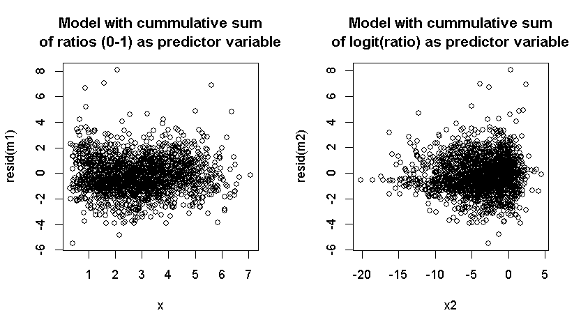
When you are transforming the predictor variables you are not really looking for/addressing heteroscedasticity but non-linearity of the response.

The GLM is composed of a linear predictor and link function. The link function is defined when you set the model (see footnote), and tells you what distribution your response is assumed to be from. For a poisson model you are saying that the $\log(Y)$ varies linearly in response to your predictor $X$.

In your single predictor case your model is basically,

$\log(Y) = \beta \sum_i X_i + c$

When you transform you are instead modelling

$\log(Y) = \beta' \sum_i \mathrm{logit}(X_i) + c$

So, it comes down to you deciding which is more likely to be "true"? There are a few ways of thinking about this.

Starting empirically, don't be too put off by the apparent widening in the right hand plot of yours. Because you have logit transformed you would expect a higher density of points in the center than the edges, so that could just be a density issue. Since what you are most looking for is a deviation from linearity (rather than heteroscedasticity), you should consider putting a simple smooth through that cloud of points and seeing what that looks like - a well fitted model should have a mean close to zero for all values of your predictors.

Because your response is the same in both set-ups you can treat this as straightforward regression comparison. I.e. imagine x1 and x2 are simply two different candidate predictors, and then answer the question, which one would I choose? A simple F-test would probably do the trick.

From a more theoretical point of view, then you can consider the interpretation of the two forms. If $X_i$ is a probability, then x2 is the sum of the log-odds - which is not something I could readily attach meaning to. On the otherhand, if $X_i$ is an amount of something, measured as a proportion of a whole, then the sum x1 is simply the total proportion. From that point of view it could make more sense to stick with the first.

A third possibility would be to average the ratios, to get back to a number between 0 and 1, and THEN take the logit. This would be treating each $X_i$ as a probability, and calculating the log-odds of the average probability.

i.e.

$\log(Y) = \beta'' \mathrm{logit} (\sum_i X_i) + c$

footnote: In your case the link function is quasi-poisson so the dispersion parameter is also fitted, but that doesn't make a difference to the question