Is regression of x on y clearly better than y on x in this case?

Question

An instrument used to measure the levels of glucose in a person's blood is monitored on a random sample of 10 people. The levels are also measured using a very accurate laboratory procedure. The instrument measure is denoted by x. The laboratory procedure measure is denoted by y.

I personally think y on x is more correct because the intention is to use the instrument readings to predict the laboratory readings. And y on x minimises the errors of such predictions.

But the answer provided was x on y.

Answer 1

Lots of lab papers, especially the instrument testing experiments, apply such x on y regression.

They argue that from the data collection in the experiment, the y conditions are controlled, and get x from the instrument reading (introducing some error in it). This is the original physical model of the experiment, so the x~y+error is more suitable.

To minimize the experiment error, sometimes, y being controlled on the same condition, then x is measured for several times (or repeated experiment). This procedure may help you to understand the logic behind them and find x~y+error more clearly.

Answer 2

As is typically the case, different analyses answer different questions. Both $Y\text{ on }X$ and $X\text{ on }Y$ could be valid here, you just want to make sure your analysis matches the question you want to answer. (For more along these lines, you may want to read my answer here: What is the difference between linear regression on Y with X and X with Y?)

You are right that if all you will want to do is predict the most likely $Y$ value given knowledge of an $X$ value, you would regress $Y\text{ on }X$. However, if you want to understand how these measures are related to each other, you might want to use an errors-in-variables approach, since you believe that there is measurement error in $X$.

On the other hand, regressing $X\text{ on }Y$ (and assuming $Y$ is perfectly error-free--a so-called gold standard) allows you to study the measurement properties of $X$. For example, you can determine if the instrument becomes biased as the true value increases (or decreases) by assessing whether the function is straight or curved.

When trying to understand the properties of a measurement instrument, understanding the nature of the measurement error is very important, and this can be done by regressing $X\text{ on }Y$. For instance, when checking for homoscedasticity, you can determine if the measurement error varies as a function of the level of the true value of the construct. It is often the case with instruments that there is more measurement error at the extremes of its range than in the middle of its applicable range (i.e., its 'sweet spot'), so you can determine this, or perhaps determine what its most appropriate range is. You can also estimate the amount of measurement error in your instrument with the root mean squared error (the residual standard deviation); of course this assumes homoscedasticity, but you can also get estimates at differing points on $Y$ via fitting a smooth function, like a spline, to the residuals.

Given these considerations, I'm guessing $X\text{ on }Y$ is better, but it certainly depends on what your goals are.

Answer 3

Prediction and Forecasting

Yes you are correct, when you view this as a problem of prediction, a Y-on-X regression will give you a model such that given a instrument measurement you can make an unbiased estimate of the accurate lab measurement, without doing the lab procedure.

Put another way, if you are just interested in $E[Y|X]$ then you want Y-on-X regression.

This may seem counter-intuitive because the error structure is not the "real" one. Assuming that the lab method is a gold standard error free method, then we "know" that the true data-generative model is

$X_i = \beta Y_i + \epsilon_i$

where $Y_i$ and $\epsilon_i$ are independent identically distribution, and $E[\epsilon]=0$

We are interested in getting the best estimate of $E[Y_i|X_i]$. Because of our independence assumption we can rearrange the above:

$Y_i = \frac{X_i - \epsilon}{\beta}$

Now, taking expectations given $X_i$ is where things get hairy

$E[Y_i|X_i] = \frac{1}{\beta} X_i - \frac{1}{\beta} E[\epsilon_i|X_i]$

The problem is the $E[\epsilon_i|X_i]$ term - is it equal to zero? It doesn't actually matter, because you can never see it, and we are only modelling linear terms (or the argument extend up to whatever terms you are modelling). Any dependence between $\epsilon$ and $X$ can simply be absorbed into the constant we are estimating.

Explicitly, without loss of generality we can let

$\epsilon_i = \gamma X_i + \eta_i$

Where $E[\eta_i|X] = 0$ by definition, so that we now have

$Y_I = \frac{1}{\beta} X_i - \frac{\gamma}{\beta} X_i - \frac{1}{\beta} \eta_i$

$Y_I = \frac{1-\gamma}{\beta} X_i - \frac{1}{\beta} \eta_i $

which satisfies all the requirements of OLS, since $\eta$ is now exogenous. It doesn't matter in the slightest that the error term also contains a $\beta$ since neither $\beta$ nor $\sigma$ are known anyway and must be estimated. We can therefore simply replace those constants with new ones and use the normal approach

$Y_I = {\alpha} X_i + \eta_i $

Notice that we have NOT estimated the quantity $\beta$ that I originally wrote down - we have built the best model we can for using X as a proxy for Y.

Instrument Analysis

The person who set you this question, clearly didn't want the answer above since they say X-on-Y is the correct method, so why might they have wanted that? Most likely they were considering the task of understanding the instrument. As discussed in Vincent's answer, if you want to know about they want the instrument behaves, the X-on-Y is the way to go.

Going back to the first equation above:

$X_i = \beta Y_i + \epsilon_i$

The person setting the question could have been thinking of calibration. An instrument is said to be calibrated when it has expectation equal to the true value - that is $E[X_i|Y_i] = Y_i$. Clearly in order to calibrate $X$ you need to find $\beta$, and so to calibrate an instrument you need to do X-on-Y regression.

Shrinkage

Calibration is an intuitively sensible requirement of an instrument, but it can also cause confusion. Notice, that even a well calibrated instrument will not be showing you the expected value of $Y$! To get $E[Y|X]$ you still need to do the Y-on-X regression, even with a well calibrated instrument. This estimate will generally look like a shrunk version of the instrument value (remember the $\gamma$ term that crept in). In particular, to get a really good estimate of $E[Y|X]$ you should include your prior knowledge of the distribution of $Y$. This then leads to concepts such as regression-to-the-mean and empirical bayes.

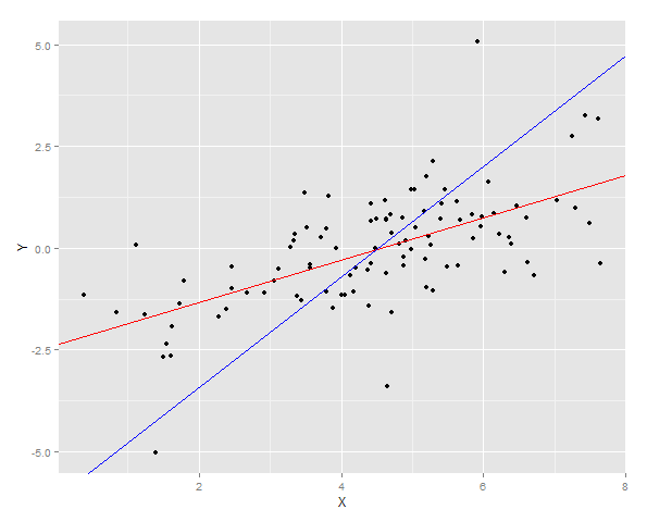
Example in R One way to get a feel for what is going on here is to make some data and try the methods out. The code below compares X-on-Y with Y-on-X for prediction and calibration and you can quickly see that X-on-Y is no good for the prediction model, but is the correct procedure for calibration.

library(data.table)
library(ggplot2)

N = 100
beta = 0.7
c = 4.4

DT = data.table(Y = rt(N, 5), epsilon = rt(N,8))
DT[, X := 0.7*Y + c + epsilon]

YonX = DT[, lm(Y~X)]   # Y = alpha_1 X + alpha_0 + eta
XonY = DT[, lm(X~Y)]   # X = beta_1 Y + beta_0 + epsilon


YonX.c = YonX$coef[1]   # c = alpha_0
YonX.m = YonX$coef[2]   # m = alpha_1

# For X on Y will need to rearrage after the fit.
# Fitting model X = beta_1 Y + beta_0
# Y = X/beta_1 - beta_0/beta_1

XonY.c = -XonY$coef[1]/XonY$coef[2]      # c = -beta_0/beta_1
XonY.m = 1.0/XonY$coef[2]  # m = 1/ beta_1

ggplot(DT, aes(x = X, y =Y)) + geom_point() +  geom_abline(intercept = YonX.c, slope = YonX.m, color = "red")  +  geom_abline(intercept = XonY.c, slope = XonY.m, color = "blue")

# Generate a fresh sample

DT2 = data.table(Y = rt(N, 5), epsilon = rt(N,8))
DT2[, X := 0.7*Y + c + epsilon]

DT2[, YonX.predict := YonX.c + YonX.m * X]
DT2[, XonY.predict := XonY.c + XonY.m * X]

cat("YonX sum of squares error for prediction: ", DT2[, sum((YonX.predict - Y)^2)])
cat("XonY sum of squares error for prediction: ", DT2[, sum((XonY.predict - Y)^2)])

# Generate lots of samples at the same Y

DT3 = data.table(Y = 4.0, epsilon = rt(N,8))
DT3[, X := 0.7*Y + c + epsilon]

DT3[, YonX.predict := YonX.c + YonX.m * X]
DT3[, XonY.predict := XonY.c + XonY.m * X]

cat("Expected value of X at a given Y (calibrated using YonX) should be close to 4: ", DT3[, mean(YonX.predict)])
cat("Expected value of X at a gievn Y (calibrated using XonY) should be close to 4: ", DT3[, mean(XonY.predict)])

ggplot(DT3) + geom_density(aes(x = YonX.predict), fill = "red", alpha = 0.5) + geom_density(aes(x = XonY.predict), fill = "blue", alpha = 0.5) + geom_vline(x = 4.0, size = 2) + ggtitle("Calibration at 4.0")

The two regression lines are plotted over the data

And then the sum of squares error for Y is measured for both fits on a new sample.

> cat("YonX sum of squares error for prediction: ", DT2[, sum((YonX.predict - Y)^2)])
YonX sum of squares error for prediction:  77.33448
> cat("XonY sum of squares error for prediction: ", DT2[, sum((XonY.predict - Y)^2)])
XonY sum of squares error for prediction:  183.0144

Alternatively a sample can be generated at a fixed Y (in this case 4) and then average of those estimates taken. You can now see that the Y-on-X predictor is not well calibrated having an expected value much lower than Y. The X-on-Y predictor, is well calibrated having an expected value close to Y.

> cat("Expected value of X at a given Y (calibrated using YonX) should be close to 4: ", DT3[, mean(YonX.predict)])
Expected value of X at a given Y (calibrated using YonX) should be close to 4:  1.305579
> cat("Expected value of X at a gievn Y (calibrated using XonY) should be close to 4: ", DT3[, mean(XonY.predict)])
Expected value of X at a gievn Y (calibrated using XonY) should be close to 4:  3.465205

The distribution of the two prediction can been seen in a density plot.

Answer 4

It depends on your assumptions about the variance of X and the variance of Y for Ordinary Least Squares. If Y has the only source of variance and X has zero variance, then use X to estimate Y. If the assumptions are the other way around (X has the only variance and Y has zero variance), then use Y to estimate X.

If both X and Y are assumed to have variance, then you may need to consider Total Least Squares.

A good description of TLS was written up at this link. The paper is geared toward trading, but section 3 does a good job of describing TLS.

Edit 1 (09/10/2013) ===============================================

I originally assumed that this was some sort of homework problem, so I didn't get real specific about "the answer" to the OP's question. But, after reading other answers, it looks like it's OK to get a little more detailed.

Quoting part of the OP's question:

"....The levels are also measured using a very accurate laboratory procedure...."

The above statement says that there are two measurements, one from the instrument and one from the lab procedure. The statement also implies that the variance for the laboratory procedure is low compared to the variance for the instrument.

Another quote from the OP's question is:

"....The laboratory procedure measure is denoted by y....."

So, from the above two statements, Y has the lower variance. So, the least error-prone technique is to use Y to estimate X. The "answer provided" was correct.